机器学习入门实践——线性回归&非线性回归&mnist手写体识别

把一本《白话深度学习与tensorflow》给啃完了，了解了一下基本的BP网络，CNN，RNN这些。感觉实际上算法本身不是特别的深奥难懂，最简单的BP网络基本上学完微积分和概率论就能搞懂，CNN引入的卷积，池化等也是数字图像处理中比较成熟的理论，RNN使用的数学工具相对而言比较高深一些，需要再深入消化消化，最近也在啃白皮书，争取从数学上把这些理论吃透

当然光学理论不太行，还是得要有一些实践的，下面是三个入门级别的，可以用来辅助对BP网络的理解

环境：win10 WSL ubuntu 18.04

1.线性回归

入门：tensorflow线性回归

https://zhuanlan.zhihu.com/p/37368943

代码：

from __future__ import  print_function
import tensorflow as tf
import numpy
import matplotlib.pyplot as plt
rng = numpy.random
# Parameters
learning_rate = 0.01
training_epochs = 1000
display_step = 50
save_step = 500
# Training Data
train_X = numpy.asarray([3.3, 4.4, 5.5, 6.71, 6.93, 4.168, 9.779, 6.182, 7.59, 2.167,
                         7.042, 10.791, 5.313, 7.997, 5.654, 9.27, 3.1])
train_Y = numpy.asarray([3, 4.7, 5, 7.21, 6.93, 4.168, 9.779, 6.182, 7.59, 2.167,
                         7.042, 10.291, 5.813, 7.997, 5.654, 9.17, 3.2])
# define graph input
X = tf.placeholder(dtype=tf.float32, name="X")
Y = tf.placeholder(dtype=tf.float32, name="Y")
with tf.variable_scope("linear_regression"):
    # set model weight
    W = tf.get_variable(initializer=rng.randn(), name="weight")
    b = tf.get_variable(initializer=rng.randn(), name="bias")
    # Construct a linear model
    mul = tf.multiply(X, W, name="mul")
    pred = tf.add(mul, b, name="pred")
# L2 loss
with tf.variable_scope("l2_loss"):
    loss = tf.reduce_mean(tf.pow(pred-Y, 2))
# Gradient descent
train_op = tf.train.GradientDescentOptimizer(learning_rate).minimize(loss)
# Initialize the variables
init_op = tf.global_variables_initializer()
# Checkpoint save path
ckpt_path = './ckpt/linear-regression-model.ckpt'
# create a saver
saver = tf.train.Saver()
# Summary save path
summary_path = './ckpt/'
# Create a summary to monitor tensors which you want to show in tensorboard
tf.summary.scalar('weight', W)
tf.summary.scalar('bias', b)
tf.summary.scalar('loss', loss)
# Merges all summaries collected in the default graph
merge_summary_op = tf.summary.merge_all()
# Start training
with tf.Session() as sess:
    summary_writer = tf.summary.FileWriter(summary_path, sess.graph)
    # Run the initializer
    sess.run(init_op)
    # Fit all training data
    for epoch in range(training_epochs):
        for (x, y) in zip(train_X, train_Y):
            # Do feed dict
            _, summary = sess.run([train_op, merge_summary_op], feed_dict={X: x, Y: y})
        if (epoch + 1) % save_step == 0:
            # Do save model
            save_path = saver.save(sess, ckpt_path, global_step=epoch)
            print("Model saved in file %s" % save_path)
        if (epoch + 1) % display_step == 0:
            # Display loss and value
            c = sess.run(loss, feed_dict={X: train_X, Y: train_Y})
            print("Epoch:", "%04d" % (epoch+1), "loss=", "{:.9f}".format(c),
                  "W=", W.eval(), "b=", b.eval())
            # Add variable state to summary file
            summary_writer.add_summary(summary, global_step=epoch)
    print("Optimization finished")
    # Save the final model
    summary_writer.close()
    # Calculate final loss after training
    training_loss = sess.run(loss, feed_dict={X: train_X, Y: train_Y})
    print("Training loss=", training_loss, "W=", sess.run(W), "b=", sess.run(b), '
')
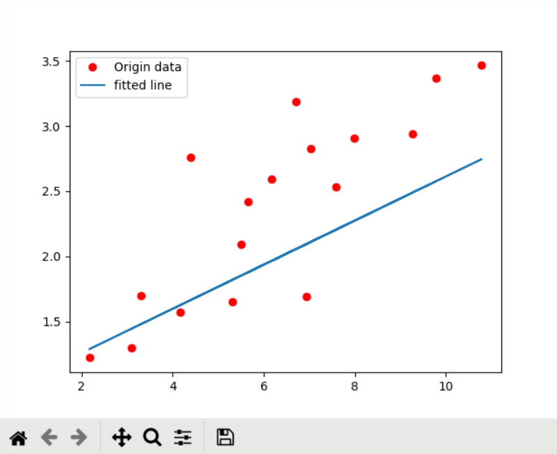
    plt.plot(train_X, train_Y, 'ro', label='Origin data')
    plt.plot(train_X, sess.run(W) * train_X + sess.run(b), label='fitted line')
    plt.legend()
    plt.show()

使用tensorboard的方法：

tensorboard --logdir=./ckpt/  (程序中存储summary的地址)

然后在浏览器输入

127.0.0.1:6006

即可查看

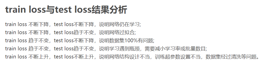
我训练的时候出现过loss不降反升的问题，说明选择的学习率有问题

除了学习率之外，学习的效果和优化算法的选择也有关系，我一开始选择的是梯度下降算法

train_op = tf.train.GradientDescentOptimizer(learning_rate).minimize(loss) 

但是效果很不好

而更换优化算法为

train_op = tf.train.AdamOptimizer(learning_rate).minimize(loss)

效果好了不少

loss也比梯度下降小了一倍多

关于各个梯度算法的介绍

https://ruder.io/optimizing-gradient-descent/index.html

https://zhuanlan.zhihu.com/p/22252270

SGD（随机梯度下降）的缺点：

由于从头至尾使用的学习率完全一致，难以选择合适的学习率

容易困于鞍点（可以通过合适的初始化和step size克服）

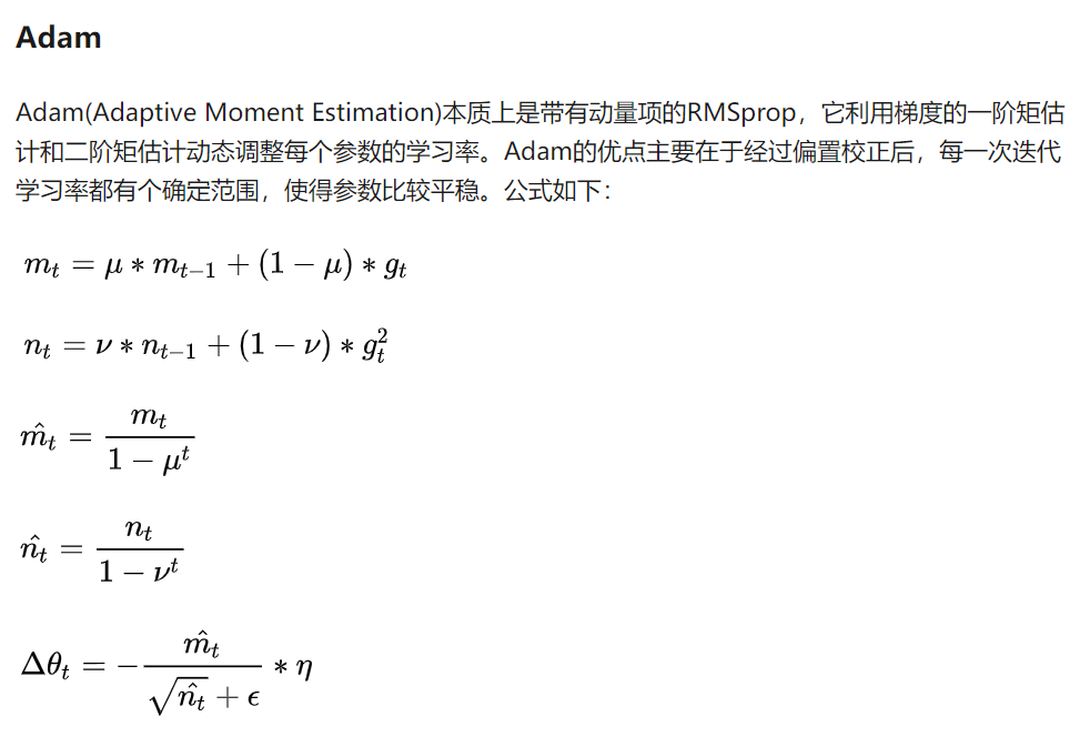
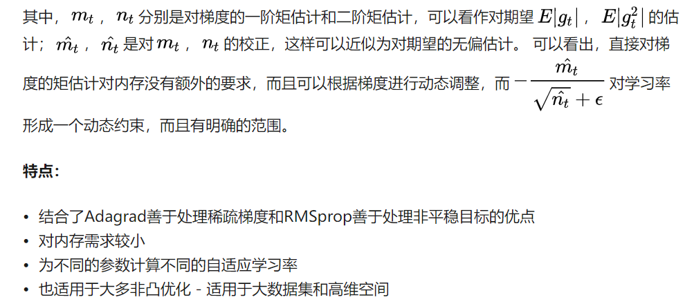
而Adam算法通过引入梯度的一阶矩和二阶矩估计，引入了近似于动量和摩擦力的物理性质，使得训练具有了自适应性，所以比单纯的梯度下降往往要好用一些。

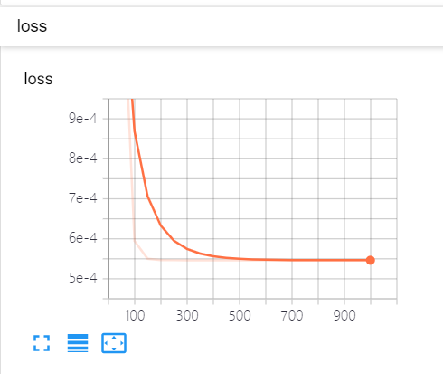
借助tensorboard可视化的观察loss，bias和weight的变化还是比较方便的，另外查看graph的功能也很好用

使用checkpoint保存的模型：

1.定义一个一模一样的graph，然后导入，可以发现创建图的过程和线性回归的代码一模一样的，创建完毕之后最关键的就是创建tf.train.Saver()，然后调用Saver类下面的restore方法，参数一个是sess一个是ckpt文件的路径

2.直接导入meta文件，这样可以将graph和参数一起导入

1.代码

from __future__ import print_function
import tensorflow as tf
import matplotlib.pyplot as plt
import numpy
rng = numpy.random
X = tf.placeholder(dtype=tf.float32, name="X")
Y = tf.placeholder(dtype=tf.float32, name="Y")
with tf.variable_scope("linear_regression"):
    W = tf.Variable(rng.randn(), name="weight")
    b = tf.Variable(rng.randn(), name="bias")
    mul = tf.multiply(X, W, name="mul")
    pred = tf.add(mul, b, name="pred")
saver = tf.train.Saver()
ckpt_path = './ckpt/linear-regression-model.ckpt-999'
with tf.Session() as sess:
    saver.restore(sess, ckpt_path)
    print('Restored Value W={}, b={}'.format(W.eval(),b.eval()))

结果：

2.代码

采用import_meta_graph导入graph，需要筑起启动Session时要设置参数config=config

调用graph中的tensor时可以直接使用graph.get_tensor_by_name

from __future__ import print_function

import tensorflow as tf

import matplotlib.pyplot as plt

import numpy

config = tf.ConfigProto(allow_soft_placement=True)

*# path of the .meta file*

ckpt = './ckpt/linear-regression-model.ckpt-999'

with tf.Session(config=config) as sess:

 saver = tf.train.import_meta_graph(ckpt + '.meta')

 saver.restore(sess, ckpt)

 graph = sess.graph

 X = graph.get_tensor_by_name("X:0")

 pred = graph.get_tensor_by_name("linear_regression/pred:0")

 

 W = graph.get_tensor_by_name("linear_regression/weight:0")

 b = graph.get_tensor_by_name("linear_regression/bias:0")

 

 print('Restored value W={}, b={}'.format(W.eval(), b.eval()))

结果：

2.非线性回归

https://blog.csdn.net/y12345678904/article/details/77743696

线性回归中使用的multiply()，但是由于实际使用中都是矩阵相乘，所以matmul更加的常用一些

tf.matmul() 和tf.multiply() 的区别

1.tf.multiply（）两个矩阵中对应元素各自相乘

格式: tf.multiply(x, y, name=None)

参数:

x: 一个类型为:half, float32, float64, uint8, int8, uint16, int16, int32, int64, complex64, complex128的张量。

y: 一个类型跟张量x相同的张量。

返回值： x * y element-wise.

注意：

（1）multiply这个函数实现的是元素级别的相乘，也就是两个相乘的数元素各自相乘，而不是矩阵乘法，注意和tf.matmul区别。

（2）两个相乘的数必须有相同的数据类型，不然就会报错。

2.tf.matmul（）将矩阵a乘以矩阵b，生成a * b。

格式: tf.matmul(a, b, transpose_a=False, transpose_b=False, adjoint_a=False, adjoint_b=False, a_is_sparse=False, b_is_sparse=False, name=None)

参数:

a: 一个类型为 float16, float32, float64, int32, complex64, complex128 且张量秩 > 1 的张量。

b: 一个类型跟张量a相同的张量。

transpose_a: 如果为真, a则在进行乘法计算前进行转置。

transpose_b: 如果为真, b则在进行乘法计算前进行转置。

adjoint_a: 如果为真, a则在进行乘法计算前进行共轭和转置。

adjoint_b: 如果为真, b则在进行乘法计算前进行共轭和转置。

a_is_sparse: 如果为真, a会被处理为稀疏矩阵。

b_is_sparse: 如果为真, b会被处理为稀疏矩阵。

name: 操作的名字（可选参数）

返回值： 一个跟张量a和张量b类型一样的张量且最内部矩阵是a和b中的相应矩阵的乘积。

注意：

（1）输入必须是矩阵（或者是张量秩 >２的张量，表示成批的矩阵），并且其在转置之后有相匹配的矩阵尺寸。

（2）两个矩阵必须都是同样的类型，支持的类型如下：float16, float32, float64, int32, complex64, complex128。

代码：

import tensorflow as tf
import numpy as np
import matplotlib.pyplot as plt
learning_rate = 0.1
training_epochs = 20000
display_step = 500
x_data = np.linspace(-1,1,200)
x_data = x_data.reshape((200,1))
noise = np.random.normal(0, 0.05, x_data.shape)
y_data = np.square(x_data) + noise
x = tf.placeholder(tf.float32, [200,1])
y = tf.placeholder(tf.float32, [200,1])
# hidden layer
weights_l1 = tf.Variable(tf.random_normal([1, 10]))
biases_l1 = tf.Variable(tf.zeros([1, 10]))
wx_plus_b_l1 = tf.matmul(x, weights_l1) + biases_l1
l1 = tf.nn.tanh(wx_plus_b_l1)
# output layer
weights_l2 = tf.Variable(tf.random_normal([10,1]))
biases_l2 = tf.Variable(tf.zeros([1,1]))
wx_plus_b_l2 = tf.matmul(l1, weights_l2) + biases_l2
prediction = tf.nn.tanh(wx_plus_b_l2)
# loss function
loss = tf.reduce_mean(tf.square(y - prediction))
# gradient descent
train_step = tf.train.GradientDescentOptimizer(learning_rate).minimize(loss)
with tf.Session() as sess:
    sess.run(tf.global_variables_initializer())
    for global_epochs in range(training_epochs):
        sess.run(train_step, feed_dict={x:x_data, y:y_data})

        if (global_epochs + 1) % display_step == 0:
            loss_value = sess.run(loss, feed_dict={x:x_data, y:y_data})
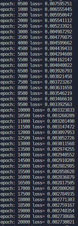
            print("epoch:", "%04d" %(global_epochs + 1), "loss=", "{:.9f}".format(loss_value)) 
    prediction_value = sess.run(prediction, feed_dict={x:x_data})
    plt.figure()
    plt.scatter(x_data, y_data)
    plt.plot(x_data, prediction_value,'r-',lw=3)
    plt.show()

结果：

下降的效果还是比较明显的，从0.0076一直下降到了0.0027

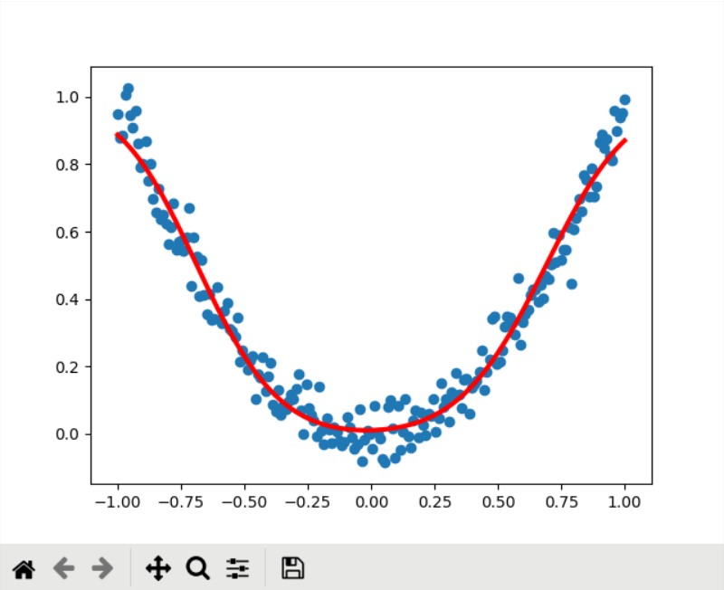
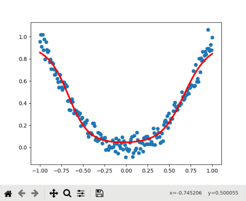
图像：

Gradient Descent的结果，比较符合二次曲线的分布规律

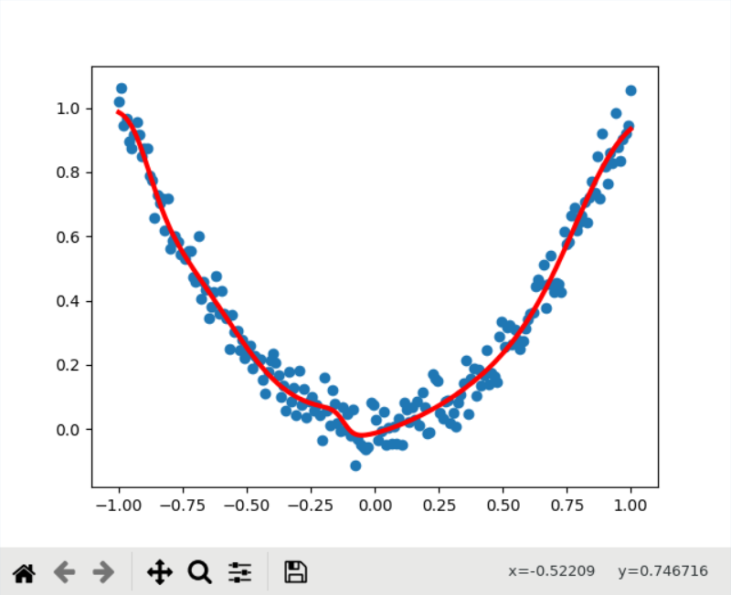
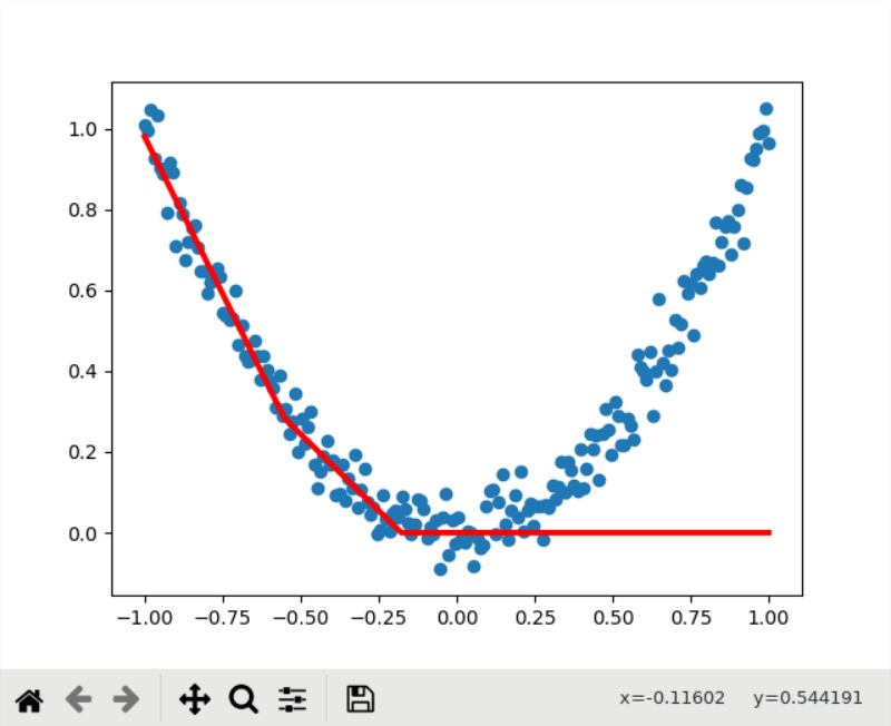
Adam的结果，虽然loss比Gradient Descent小，但是实际上有比较明显的过拟合了

另外这里的激活函数采用的是tanh，更换成sigmoid之后

效果差于tanh做激活函数，因为tanh的导数值大于sigmoid，收敛速度实际上是快于sigmoid的，不过我把训练次数翻到了40000次后发现好像sigmoid作为激活函数，训练的上限就是0.004几了，而如果采用ReLU的话，就直接起飞了，根本无法收敛

ReLU还是适合在深度网络中做激活函数，在这种就一层的网络里面来搞效果就比较差（本来的目的就是为了解决深度网络中的梯度爆炸）

3.全连接网络实例（mnist）

https://geektutu.com/post/tensorflow-mnist-simplest.html

分为一个mnist_model.py用于构建网络，一个mnist_train.py用于训练，这种构建方式是大多数神经网络都会采取的方式

一维向量既可以用[1, 维数]来表示，也可以用[None, 维数]来表示

l由于label采用了1-10的独热编码，loss函数使用的是交叉熵，公式为（p为真实分布，q为非真实分布）

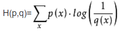
代码为

self.loss = -tf.reduce_sum(self.label * tf.log(self.y + 1e-10))

这里加1e-10的目的是为了防止y=0时出现数值溢出错误

关于feed_dict
sess.run() 中的feed_dict

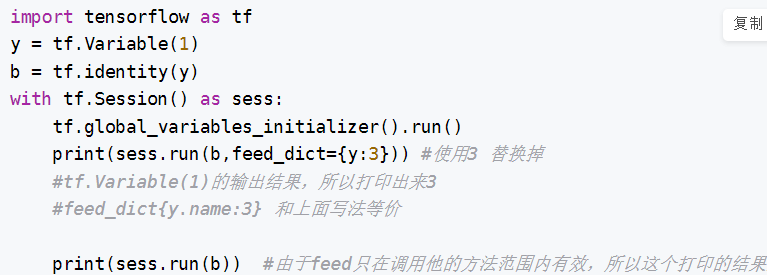
结果是1，本质上就是一个临时赋值的功能

model的代码：

import tensorflow as tf
class Network:
    def __init__(self):
        # learning rate
        self.learning_rate = 0.01
        # input tensor
        self.x = tf.placeholder(tf.float32, [None, 784])
        # label tensor
        self.label = tf.placeholder(tf.float32, [None, 10])
        # weight
        self.w = tf.Variable(tf.random_normal([784, 10]))
        # bias
        self.b = tf.Variable(tf.random_normal([10]))
        # output tensor
        self.y = tf.nn.softmax(tf.matmul(self.x, self.w) + self.b)
        # loss
        self.loss = -tf.reduce_sum(self.label * tf.log(self.y + 1e-10))
        # train
        self.train = tf.train.GradientDescentOptimizer(self.learning_rate).minimize(self.loss)
        # verify
        predict = tf.equal(tf.arg_max(self.label, 1), tf.arg_max(self.y, 1))
        # calc the accuracy
        self.accuracy = tf.reduce_mean(tf.cast(predict, "float"))

train的代码:

train的代码
import tensorflow as tf
from tensorflow.examples.tutorials.mnist import input_data
from mnist_model import Network
class Train:
    def __init__(self):
        self.net = Network()
        # initialize session
        self.sess = tf.Session()
        # initialize variables
        self.sess.run(tf.global_variables_initializer())
        # input data
        self.data = input_data.read_data_sets('/home/satori/python/tensorflow_test/data_set', one_hot=True)
        # create a saver
        self.saver = tf.train.Saver()
    def train(self):
        batch_size = 64
        train_epoch = 10000
        save_interval = 1000
        display_interval = 100
        ckpt_path = './ckpt/mnist-model.ckpt'
        for step in range(train_epoch):
            x, label = self.data.train.next_batch(batch_size)
            # training
            self.sess.run(self.net.train, feed_dict={self.net.x:x, self.net.label:label})
            if (step + 1) % display_interval == 0:
                # print the loss
                loss = self.sess.run(self.net.loss, feed_dict={self.net.x:x, self.net.label:label})
                print("step=%d, loss=%.2f" %((step+1), loss))
            
            if (step + 1) % save_interval == 0:
                # save the model
                self.saver.save(self.sess, ckpt_path, global_step=step)
                print("model saved in file %s" %ckpt_path)

    def calculate_accuracy(self):
        test_x = self.data.test.images
        test_label = self.data.test.labels
        # using the net trained
        accuracy = self.sess.run(self.net.accuracy, feed_dict={self.net.x: test_x, self.net.label: test_label})
        print("accuracy=%.2f,%dof pictures are tested" %(accuracy,len(test_label)))
    
if __name__ == "__main__":
    app = Train()
    app.train()
    app.calculate_accuracy()

train中会保存模型，然后我们需要将模型导入predict，对样本进行识别

import numpy as np
import tensorflow as tf
from PIL import Image
from mnist_model import Network
ckpt_path = './ckpt/mnist-model.ckpt-9999'
class Predict:
    def __init__(self):
        # restore the network
        self.net = Network()
        self.sess = tf.Session()
        self.sess.run(tf.global_variables_initializer())
        self.restore()
    def restore(self):
        saver = tf.train.Saver()
        saver.restore(self.sess, ckpt_path)
    def predict(self, image_path):
        # turn image into black and white
        img = Image.open(image_path).convert('L')
        flatten_img = np.reshape(img, 784)
        x = np.array([1 - flatten_img])
        y = self.sess.run(self.net.y, feed_dict={self.net.x: x})
        
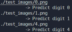
        print(image_path)
        print('          -> Predict digit', np.argmax(y[0]))
if __name__ == "__main__":
    app = Predict()
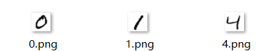
    app.predict('./test_images/0.png')
    app.predict('./test_images/1.png')
    app.predict('./test_images/4.png')

样本：

运行结果：

另外在导入模型方面，还可以引入

def restore(self):
        saver = tf.train.Saver()
        ckpt = tf.train.get_checkpoint_state(CKPT_DIR)
        if ckpt and ckpt.model_checkpoint_path:
            saver.restore(self.sess, ckpt.model_checkpoint_path)
        else:
            raise FileNotFoundError("未保存任何模型")

进行错误处理

实际上还是可以像线性回归那边一样加入一个summary来方便用tensorboard来可视化，不过因为我上面跑的还挺成功的，就先不搞这个了，总体上还是比较顺利的