机器学习

案例背景 

银行评判用户的信用考量规避信用卡诈骗

▒ 数据

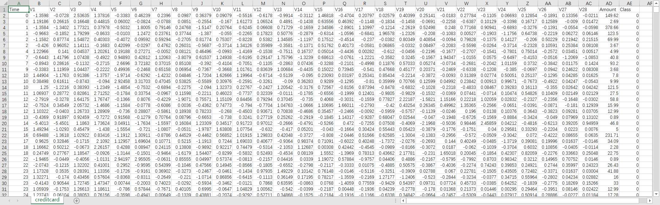
数据共有 31 个特征, 为了安全起见数据已经向了模糊化处理无法读出真实信息目标

其中数据中的 class 特征标识为是否正常用户 (0 代表正常, 1 代表异常)

▒ 目标

本质依旧是一个分类问题, 0/1 的问题判断是否为信用卡诈骗用户

而在数据中 class 已经进行标识, 而且这次的样本数据的两项结果是极度的不均衡

既正常用户的样本数量是远远大于异常数据的.

不均衡的数据处理方式可以进行 下采样, 或者上采样

▨ 下采样 -  对多的数据进行消减到和少的数据一样少

▨ 上采样 -  对少的数据进行填充到和多的数据一样多

案例统计

▒ 准备 - 三件套

import pandas as pd
import matplotlib.pyplot as plt
import numpy as np

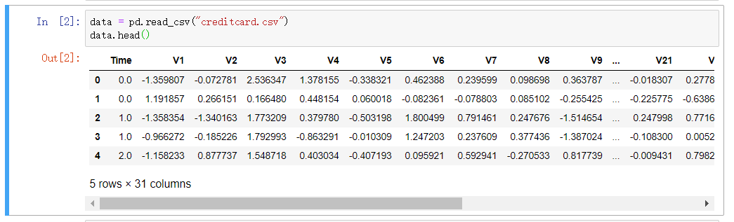
▒ 样本数据查看 

▒ 异常数量统计

count_classes = pd.value_counts(data['Class'], sort = True).sort_index()  # 某一列的查询按照数据排序
count_classes.plot(kind = 'bar') # 条形图
plt.title("Fraud class histogram") # 标题
plt.xlabel("Class") # x 轴
plt.ylabel("Frequency") # y 轴

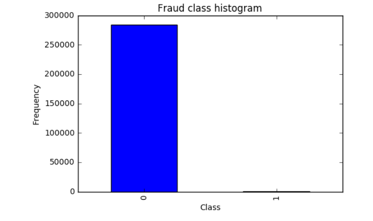
可以看出正常用户多达28w, 而异常样本大概有几百个左右, 

数据预处理 - 标准化

▒ 概念  

机器学习的常规认知是对较大的特征数值基于更大的影响, 因此当特征的的取值大小之间的不同,

会导致认为较大数值的特征比较小数值特征的影响更大, 因此需要对数据特征进行归一化处理

比如都限制在取值在 0-1 之间这样机器学习会将所有的特征按照统一的标准进行考量

▒ 操作代码 

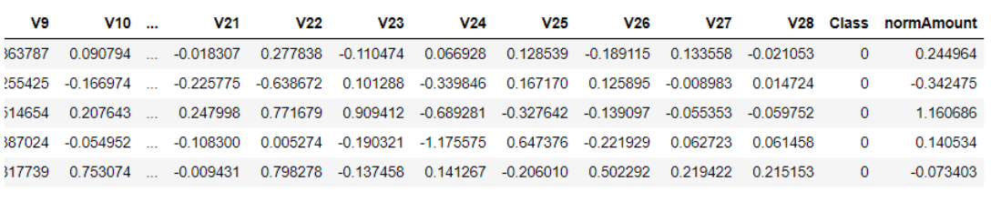
from sklearn.preprocessing import StandardScaler 

data['normAmount'] = StandardScaler().fit_transform(data['Amount'].reshape(-1, 1))
data = data.drop(['Time','Amount'],axis=1)
data.head()

▨ 详解

引用  sklearn  模块进行预处理操作

reshape  方法进行维度的重处理

　　取值  (-1, 1)  中的 -1 表示系统自动判断, 后面是提供参考值 (  比如原来是 2,3 的维度,  你输入 (-1,1) 则表示转换为  ( 6,1 ), 系统对 -1 进行自动计算 )

然后生成的新特征填充到样本数据中, 删除掉转换前的特征, 以及没有用的特征

 fit_transform  对数据进行归一化处理, 具体流程为先拟合后进行归一处理

下采样

▒ 概念

下采样的方法为将多的那类数据样本降和少的那类一样的少

▨ 操作代码

from sklearn.linear_model import LogisticRegression # 逻辑回归计算
from sklearn.model_selection import KFold # 交叉验证计算
from sklearn.model_selection import cross_val_score 
from sklearn.metrics import confusion_matrix 
from sklearn.metrics import recall_score # 召回率计算
from sklearn.metrics import classification_report

X = data.ix[:, data.columns != 'Class'] # 除了 "Class" 列的其他列的所有数据
y = data.ix[:, data.columns == 'Class'] # "Class" 列的数据

number_records_fraud = len(data[data.Class == 1]) # 所有的异常(class == 1)的数据的个数
fraud_indices = np.array(data[data.Class == 1].index) # 所有的异常(class == 1)的数据的索引

normal_indices = data[data.Class == 0].index # 所有的正常(class == 0)数据的索引

# np 的随机模块进行选择 参数:( 被选容器(正常数据), 个数(异常数据个数), 是否代替(不代替) )
random_normal_indices = np.random.choice(normal_indices, number_records_fraud, replace = False)
random_normal_indices = np.array(random_normal_indices)

# 拼接数组
under_sample_indices = np.concatenate([fraud_indices,random_normal_indices])

# 下采样之后的数据
under_sample_data = data.iloc[under_sample_indices,:]

# X , y 
X_undersample = under_sample_data.ix[:, under_sample_data.columns != 'Class']
y_undersample = under_sample_data.ix[:, under_sample_data.columns == 'Class']

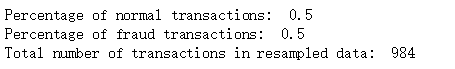
将异常数据的个数计算出来后, 然后在政策数据集中随机筛选出异常数据集个数的数据, 然后组合为新的数据集

从而保证异常数据集和正常数据集为 1:1 比例

▨ 结果

# Showing ratio
print("Percentage of normal transactions: ", len(under_sample_data[under_sample_data.Class == 0])/len(under_sample_data))
print("Percentage of fraud transactions: ", len(under_sample_data[under_sample_data.Class == 1])/len(under_sample_data))
print("Total number of transactions in resampled data: ", len(under_sample_data))

▒ 交叉验证

▨ 概念

数据集在最开始的时候会划分为 训练集 和 测试集

训练集用于建模, 测试集用于对模型进行验证

而建模阶段训练集通常会进行 n 等分, 然后彼此再次划分 训练集和测试集

目的是为了获取正确的参数, 从而需要进行多次的训练集和测试集的互换从而交叉验证 

▨ 划分数据集

from sklearn.model_selection import train_test_split

# 原始数据集切分数据 - 0.3 的测试集, 0.7 的训练集 , 设定随机参数
X_train, X_test, y_train, y_test = train_test_split(X,y,test_size = 0.3, random_state = 0) # 

print("Number transactions train dataset: ", len(X_train))
print("Number transactions test dataset: ", len(X_test))
print("Total number of transactions: ", len(X_train)+len(X_test))

# 下采样数据集切分数据 - 0.3 的测试集, 0.7 的训练集 , 设定随机参数
X_train_undersample, X_test_undersample, y_train_undersample, y_test_undersample = train_test_split(X_undersample
                                                                                                   ,y_undersample
                                                                                                   ,test_size = 0.3
                                                                                                   ,random_state = 0)
print("")
print("Number transactions train dataset: ", len(X_train_undersample))
print("Number transactions test dataset: ", len(X_test_undersample))
print("Total number of transactions: ", len(X_train_undersample)+len(X_test_undersample))

评估方法

▒ 精度

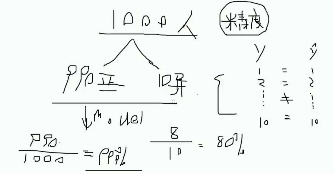
通常的评估方法中可以使用精度计算

精度计算的评估方法很大程度取决于样本数据本身的情况

尤其是不对称的数据中会造成精度计算的极大不准确性

如图所示, 如1000 数据中 990 数据为正样本数据, 则计算出的结果则为 99.9% 则负样本预测不出来. 实则无用

▒ Recall 

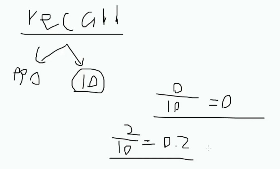
根据目标来指定标准, 比如 1000数据中的异常数据为 10 , 目标则是找出异常数据

则根据检测出的异常数据于原有的异常数据进行比对来判断计算 recall 值

▨ 概念

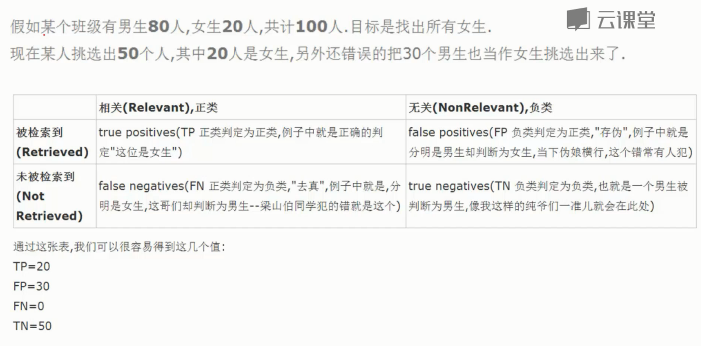
　　两个维度, 1 是否符合预期 (P/N) , 2 判断是否正确 (T/F)

• TP - 目标找女生, 找出女生判断是女生 - 符合预期 ( 正例 ),  正确判断
• FP - 目标找女生, 找出男生判断为女生 - 符合预期 ( 正例 ),  错误判断
• FN - 目标找女生, 找出女生判断为男生 - 不符合预期 ( 负例 ),  错误判断
• TN - 目标找女生, 找出男生判断为男生 - 不符合预期 ( 负例 ),  正确判断

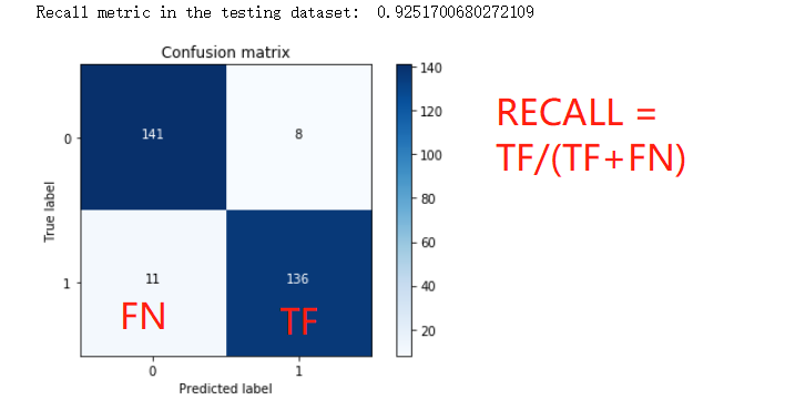
▨ 公式

Recall = TP/(TP+FN)

正则化惩罚

▒ 概念 

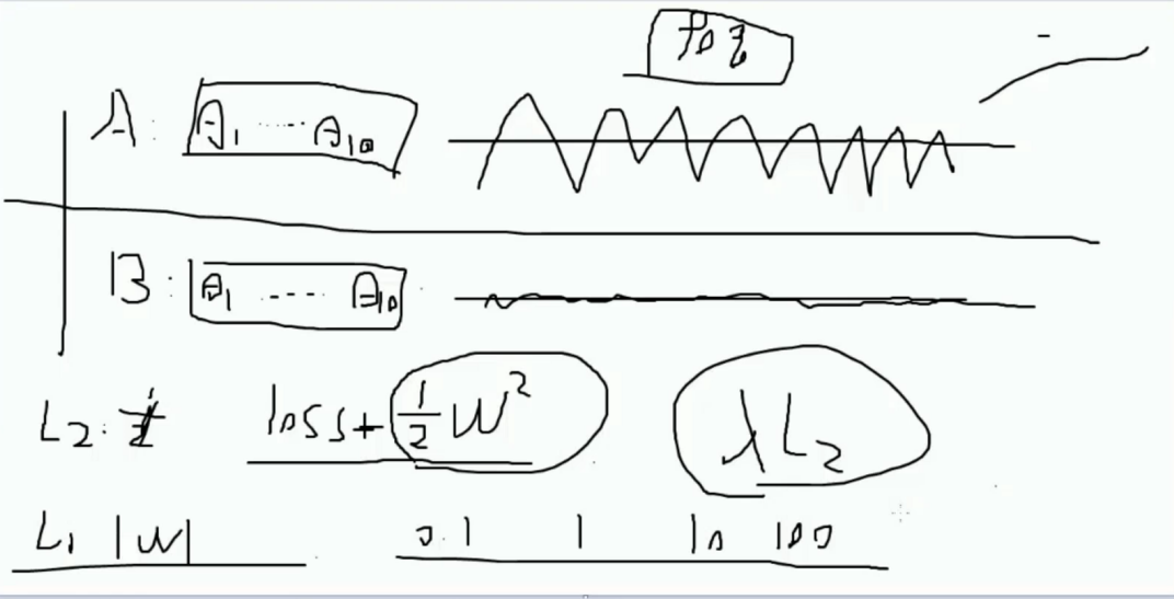
在不同的模型中可能存在最终的 Recall 都一样的情况, 如果 Recall 相同的是否可以理解为两个模型效果相同?

但是模型本质可能还是存在不同, 因此需要在另一个维度进行分析, 图示的 A 和 B 的参数可见其实是不同的

A 的浮动明显很大, B 的浮动小很多, 浮动过大可能是过拟合的问题导致, 而此时引入一个惩罚概念进行筛选

对浮动过大的进行惩罚更大, 由此进行区分, 惩罚方式可以选择 L1/L2 等, 具体的原酸都是加入一个值进行区分

而惩罚粒度也可以限制从  0.1 ,1,10,100 不等, 而这个粒度则需要交叉验证进行选择, 既比对参数 

▒ 操作代码

def printing_Kfold_scores(x_train_data,y_train_data):
    fold = KFold(5,shuffle=False) # 划分为 5 等分, 即 5次交叉验证, shuffle 不洗牌

    # 默认的惩罚粒度参数容器
    c_param_range = [0.01,0.1,1,10,100]
    
    # 展示用
    results_table = pd.DataFrame(index = range(len(c_param_range),2), columns = ['C_parameter','Mean recall score'])
    results_table['C_parameter'] = c_param_range

    # the k-fold will give 2 lists: train_indices = indices[0], test_indices = indices[1]
    j = 0
    for c_param in c_param_range: # 循环每个待选参数
    
        print('-------------------------------------------')
        print('C parameter: ', c_param)
        print('-------------------------------------------')
        print('')

        recall_accs = []
        for iteration, indices in enumerate(fold.split(x_train_data)): # 交叉验证

            # 建立逻辑回归模型实例化, 传入惩罚项粒度, 以及惩罚模式 可以选择 l1 或者 l2 
            # solver='liblinear' 是为了避免 FutureWarning 提示
            lr = LogisticRegression(C = c_param, penalty = 'l1',solver='liblinear')

            # 训练模型 
            lr.fit(x_train_data.iloc[indices[0],:],y_train_data.iloc[indices[0],:].values.ravel())
            
            # 预测
            y_pred_undersample = lr.predict(x_train_data.iloc[indices[1],:].values)

            # 计算召回率
            recall_acc = recall_score(y_train_data.iloc[indices[1],:].values,y_pred_undersample)
            recall_accs.append(recall_acc)
            print('Iteration ', iteration,': recall score = ', recall_acc)

        # 计算均值展示
        results_table.loc[j,'Mean recall score'] = np.mean(recall_accs)
        j += 1
        print('')
        print('Mean recall score ', np.mean(recall_accs))
        print('')

    best_c = results_table.loc[results_table['Mean recall score'].values.argmax()]['C_parameter']
    
    # 打印最好的选择
    print('*********************************************************************************')
    print('Best model to choose from cross validation is with C parameter = ', best_c)
    print('*********************************************************************************')
    
    return best_c

▒  测试结果

best_c = printing_Kfold_scores(X_train_undersample,y_train_undersample)

 打印结果对比可以看出 经过了5次不洗牌的交叉验证后,  为 0.01 的 recall 值最高, 为最优参数

-------------------------------------------
C parameter:  0.01
-------------------------------------------

Iteration  0 : recall score =  0.958904109589041
Iteration  1 : recall score =  0.9178082191780822
Iteration  2 : recall score =  1.0
Iteration  3 : recall score =  0.9594594594594594
Iteration  4 : recall score =  0.9848484848484849

Mean recall score  0.9642040546150135

-------------------------------------------
C parameter:  0.1
-------------------------------------------

Iteration  0 : recall score =  0.8493150684931506
Iteration  1 : recall score =  0.863013698630137
Iteration  2 : recall score =  0.9152542372881356
Iteration  3 : recall score =  0.918918918918919
Iteration  4 : recall score =  0.8939393939393939

Mean recall score  0.8880882634539471

-------------------------------------------
C parameter:  1
-------------------------------------------

Iteration  0 : recall score =  0.863013698630137
Iteration  1 : recall score =  0.863013698630137
Iteration  2 : recall score =  0.9661016949152542
Iteration  3 : recall score =  0.9459459459459459
Iteration  4 : recall score =  0.9090909090909091

Mean recall score  0.9094331894424765

-------------------------------------------
C parameter:  10
-------------------------------------------

Iteration  0 : recall score =  0.863013698630137
Iteration  1 : recall score =  0.863013698630137
Iteration  2 : recall score =  0.9830508474576272
Iteration  3 : recall score =  0.9324324324324325
Iteration  4 : recall score =  0.9242424242424242

Mean recall score  0.9131506202785514

-------------------------------------------
C parameter:  100
-------------------------------------------

Iteration  0 : recall score =  0.863013698630137
Iteration  1 : recall score =  0.863013698630137
Iteration  2 : recall score =  0.9830508474576272
Iteration  3 : recall score =  0.9324324324324325
Iteration  4 : recall score =  0.9242424242424242

Mean recall score  0.9131506202785514

*********************************************************************************
Best model to choose from cross validation is with C parameter =  0.01
*********************************************************************************

▨ 对比正常数据直接操作

best_c = printing_Kfold_scores(X_train,y_train)

-------------------------------------------
C parameter:  0.01
-------------------------------------------

Iteration  0 : recall score =  0.4925373134328358
Iteration  1 : recall score =  0.6027397260273972
Iteration  2 : recall score =  0.6833333333333333
Iteration  3 : recall score =  0.5692307692307692
Iteration  4 : recall score =  0.45

Mean recall score  0.5595682284048672

-------------------------------------------
C parameter:  0.1
-------------------------------------------

Iteration  0 : recall score =  0.5671641791044776
Iteration  1 : recall score =  0.6164383561643836
Iteration  2 : recall score =  0.6833333333333333
Iteration  3 : recall score =  0.5846153846153846
Iteration  4 : recall score =  0.525

Mean recall score  0.5953102506435158

-------------------------------------------
C parameter:  1
-------------------------------------------

Iteration  0 : recall score =  0.5522388059701493
Iteration  1 : recall score =  0.6164383561643836
Iteration  2 : recall score =  0.7166666666666667
Iteration  3 : recall score =  0.6153846153846154
Iteration  4 : recall score =  0.5625

Mean recall score  0.612645688837163

-------------------------------------------
C parameter:  10
-------------------------------------------

Iteration  0 : recall score =  0.5522388059701493
Iteration  1 : recall score =  0.6164383561643836
Iteration  2 : recall score =  0.7333333333333333
Iteration  3 : recall score =  0.6153846153846154
Iteration  4 : recall score =  0.575

Mean recall score  0.6184790221704963

-------------------------------------------
C parameter:  100
-------------------------------------------

Iteration  0 : recall score =  0.5522388059701493
Iteration  1 : recall score =  0.6164383561643836
Iteration  2 : recall score =  0.7333333333333333
Iteration  3 : recall score =  0.6153846153846154
Iteration  4 : recall score =  0.575

Mean recall score  0.6184790221704963

*********************************************************************************
Best model to choose from cross validation is with C parameter =  10.0
*********************************************************************************

可以看出在不均衡的数据中的计算recall 值是相当糟糕

只有 0.61 和 经过下采样的计算 0.91 相差甚远

混淆矩阵

▒ 概念

混淆矩阵用来更直观的平面展示模型的情况以方便评估

这里再拉回来之前的评估方法公式回忆一下

Recall = TP/(TP+FN)

▒ 操作代码

def plot_confusion_matrix(cm, classes,
                          title='Confusion matrix',
                          cmap=plt.cm.Blues):
    """
    This function prints and plots the confusion matrix.
    """
    plt.imshow(cm, interpolation='nearest', cmap=cmap)
    plt.title(title)
    plt.colorbar()
    tick_marks = np.arange(len(classes))
    plt.xticks(tick_marks, classes, rotation=0)
    plt.yticks(tick_marks, classes)

    thresh = cm.max() / 2.
    for i, j in itertools.product(range(cm.shape[0]), range(cm.shape[1])):
        plt.text(j, i, cm[i, j],
                 horizontalalignment="center",
                 color="white" if cm[i, j] > thresh else "black")

    plt.tight_layout()
    plt.ylabel('True label')
    plt.xlabel('Predicted label')

▨ 测试结果

import itertools
lr = LogisticRegression(C = best_c, penalty = 'l1',solver='liblinear')
lr.fit(X_train_undersample,y_train_undersample.values.ravel())
y_pred_undersample = lr.predict(X_test_undersample.values)

# Compute confusion matrix
cnf_matrix = confusion_matrix(y_test_undersample,y_pred_undersample)
np.set_printoptions(precision=2)

print("Recall metric in the testing dataset: ", cnf_matrix[1,1]/(cnf_matrix[1,0]+cnf_matrix[1,1]))

# Plot non-normalized confusion matrix
class_names = [0,1]
plt.figure()
plot_confusion_matrix(cnf_matrix
                      , classes=class_names
                      , title='Confusion matrix')
plt.show()

应用实际数据集

以上是在下采样的数据集上进行的测试, 还需要在原始的数据集上进行测试才行

而在全量数据集的在进行判断才看是否精准才可以判断模型的可行性

▨ 操作代码

lr = LogisticRegression(C = best_c, penalty = 'l1',solver='liblinear')
lr.fit(X_train_undersample,y_train_undersample.values.ravel())
y_pred = lr.predict(X_test.values)

# Compute confusion matrix
cnf_matrix = confusion_matrix(y_test,y_pred)
np.set_printoptions(precision=2)

print("Recall metric in the testing dataset: ", cnf_matrix[1,1]/(cnf_matrix[1,0]+cnf_matrix[1,1]))

# Plot non-normalized confusion matrix
class_names = [0,1]
plt.figure()
plot_confusion_matrix(cnf_matrix
                      , classes=class_names
                      , title='Confusion matrix')
plt.show()

▨ 测试结果

通过测试结果就可以看出异常了,  TP (  正例判对 ) 问题不大

但是 问题是 FP ( 正例判错 ) 高达到 8000 就明显说不过去了 - 判断正常用户为诈骗犯, 误杀

这个的数据异常确实不会影响到 recall 的计算

因为  recall 值和 TP 和 FN ( 反例正判 ) 有关

因此这个的结果会对精度有一定的影响, 这也是下采样的弊端

调整阈值

在默认的回归模型中的阈值为 0.5 , 即比例完全均分的判断, 

而阈值调整提升则可以让检测更加严格, 反之更加容易通过

应用于此实例中则为

0.99 ----  不像是个诈骗犯的要死的程度是不会认为这人是诈骗犯

0.01 ----- 特么稍微有点异常动作你就是个诈骗犯了

▒ 操作代码

lr = LogisticRegression(C = 0.01, penalty = 'l1',solver='liblinear')
lr.fit(X_train_undersample,y_train_undersample.values.ravel())
y_pred_undersample_proba = lr.predict_proba(X_test_undersample.values) # 此函数产出的是概率值

thresholds = [0.1,0.2,0.3,0.4,0.5,0.6,0.7,0.8,0.9]

plt.figure(figsize=(10,10))

j = 1
for i in thresholds:
    y_test_predictions_high_recall = y_pred_undersample_proba[:,1] > i
    
    plt.subplot(3,3,j)
    j += 1
    
    # Compute confusion matrix
    cnf_matrix = confusion_matrix(y_test_undersample,y_test_predictions_high_recall)
    np.set_printoptions(precision=2)

    print("Recall metric in the testing dataset: ", cnf_matrix[1,1]/(cnf_matrix[1,0]+cnf_matrix[1,1]))

    # Plot non-normalized confusion matrix
    class_names = [0,1]
    plot_confusion_matrix(cnf_matrix
                          , classes=class_names
                          , title='Threshold >= %s'%i) 

▨ 测试结果

可见在 0.1 时 ,recall 值很高, 但是 精度很低, 因为将所有的都预测成了诈骗犯, 因此错杀很多

但是在 0.9 时 ,recall 值很低, 错杀问题解决了. 无法检测到的却很多了.

由此可见, 结合实际考虑之后, 大概在 0.5 - 0.7 之间的较为合适,

当然一般也会提供数据要求误杀率不能高于多少, 精度要大于多少, recall 要大于多少之类的, 再结合模型进行适当的选择

过采样

▒ 概念

过 ( 上 ) 采样的方法为将少的那类数据样本增加的和多的那类一样的多

▒ 代码实现

▨ 所需包引入

不同于sklearn模块,  imblearn 是需要额外自己手动安装的包   pip install imblearn 

import pandas as pd
from imblearn.over_sampling import SMOTE
from sklearn.ensemble import RandomForestClassifier
from sklearn.metrics import confusion_matrix
from sklearn.model_selection import train_test_split

▨ 具体代码

credit_cards=pd.read_csv('creditcard.csv') 

columns=credit_cards.columns 
# 去掉最后一行没用的数据
features_columns=columns.delete(len(columns)-1) 

features=credit_cards[features_columns]
labels=credit_cards['Class']

拆分训练集和测试集

features_train, features_test, labels_train, labels_test = train_test_split(features, 
                                                                            labels, 
                                                                            test_size=0.2, 
                                                                            random_state=0)

过采样数据处理

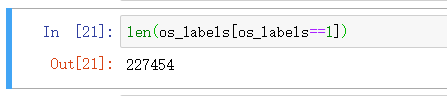
oversampler=SMOTE(random_state=0) # 指定每次生成数据相同, random_state=0
os_features,os_labels=oversampler.fit_sample(features_train,labels_train) # 那训练集进行数据的生成, 不要动测试集

可以看出数据进行了填充

 

▒ 测试结果

计算最优参数

os_features = pd.DataFrame(os_features)
os_labels = pd.DataFrame(os_labels)
best_c = printing_Kfold_scores(os_features,os_labels)

-------------------------------------------
C parameter:  0.01
-------------------------------------------

Iteration  1 : recall score =  0.890322580645
Iteration  2 : recall score =  0.894736842105
Iteration  3 : recall score =  0.968861347792
Iteration  4 : recall score =  0.957595541926
Iteration  5 : recall score =  0.958430881173

Mean recall score  0.933989438728

-------------------------------------------
C parameter:  0.1
-------------------------------------------

Iteration  1 : recall score =  0.890322580645
Iteration  2 : recall score =  0.894736842105
Iteration  3 : recall score =  0.970410534469
Iteration  4 : recall score =  0.959980655302
Iteration  5 : recall score =  0.960178498807

Mean recall score  0.935125822266

-------------------------------------------
C parameter:  1
-------------------------------------------

Iteration  1 : recall score =  0.890322580645
Iteration  2 : recall score =  0.894736842105
Iteration  3 : recall score =  0.970454796946
Iteration  4 : recall score =  0.96014552489
Iteration  5 : recall score =  0.960596168431

Mean recall score  0.935251182603

-------------------------------------------
C parameter:  10
-------------------------------------------

Iteration  1 : recall score =  0.890322580645
Iteration  2 : recall score =  0.894736842105
Iteration  3 : recall score =  0.97065397809
Iteration  4 : recall score =  0.960343368396
Iteration  5 : recall score =  0.960530220596

Mean recall score  0.935317397966

-------------------------------------------
C parameter:  100
-------------------------------------------

Iteration  1 : recall score =  0.890322580645
Iteration  2 : recall score =  0.894736842105
Iteration  3 : recall score =  0.970543321899
Iteration  4 : recall score =  0.960211472725
Iteration  5 : recall score =  0.960903924995

Mean recall score  0.935343628474

*********************************************************************************
Best model to choose from cross validation is with C parameter =  100.0
*********************************************************************************

 可以看出 100 为最优选择

 继续计算混淆矩阵

lr = LogisticRegression(C = best_c, penalty = 'l1')
lr.fit(os_features,os_labels.values.ravel())
y_pred = lr.predict(features_test.values)

# Compute confusion matrix
cnf_matrix = confusion_matrix(labels_test,y_pred)
np.set_printoptions(precision=2)

print("Recall metric in the testing dataset: ", cnf_matrix[1,1]/(cnf_matrix[1,0]+cnf_matrix[1,1]))

# Plot non-normalized confusion matrix
class_names = [0,1]
plt.figure()
plot_confusion_matrix(cnf_matrix
                      , classes=class_names
                      , title='Confusion matrix')
plt.show()

 

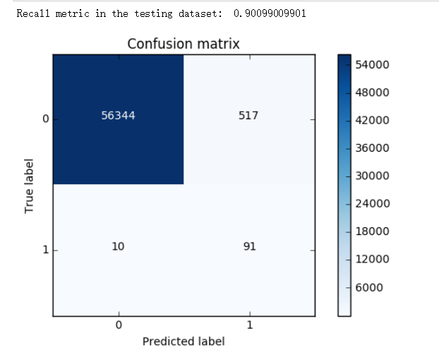
 由结果可以看出.

尽管 Recall 值相对较低, 不如下采样的高

但是 误杀的程度要低很多. 只有 517 个, 比起下采样的 8000个要好很多

而精度当然也是 过采样 更好一些

总结

▒ 流程

▨ 观察数据

观察数据的特征 - 标准化处理/特征工程

观察数据的分布 - 是否均衡 - 不均衡的话怎么处理 - 下采样/过采样

下采样和过采样的选择问题

　　优先还是选择过采样. 尽管下采样的 Recall 更高

　　但是数据量越大对于模型的稳定性是越高的, 由此也更可靠.

　　因此比起削减数据. 增加数据是更好的选择

▨ 计算参数选择

交叉验证计算 Recall 比对选择最合适的参数

▨ 阈值选择

逻辑回归中的阈值选择

▨ 评估

根据混淆矩阵, 计算 TP / FP / TN / FN / Recall / 精度