在使用多目标跟踪算法时,接触到卡尔曼滤波,一直没时间总结下,现在来填坑。。
1. 背景知识
在理解卡尔曼滤波前,有几个概念值得考虑下:时序序列模型,滤波,线性动态系统
1. 时间序列模型
时间序列模型都可以用如下示意图表示:
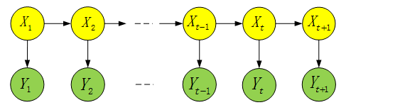
这个模型包含两个序列,一个是黄色部分的状态序列,用X表示,一个是绿色部分的观测序列(又叫测量序列、证据序列、观察序列,不同的书籍有不同的叫法,在这里统一叫观测序列。)用Y表示。状态序列反应了系统的真实状态,一般不能被直接观测,即使被直接观测也会引进噪声;观测序列是通过测量得到的数据,它与状态序列之间有规律性的联系。
上面序列中,假设初始时间为(t_1), 则(X_1,Y_1)是(t_1)时刻的状态值和观测值,(X_2,Y_2)是(t_2)时刻的状态值和观测值...,即随着时间的流逝,序列从左向右逐渐展开。
常见的时间序列模型主要包括三个:隐尔马尔科夫模型,卡尔曼滤波,粒子滤波。
2. 滤波
时间序列模型中包括预测和滤波两步
- 预测:指用当前和过去的数据来求取未来的数据。对应上述序列图中,则是利用(t_1)时刻(X_1,Y_1)的值,估计(t_2)时刻(X_2)值。
- 滤波:是用当前和过去的数据来求取当前的数据。对应上述序列图中,则是先通过上一步的预测步骤得到(X_2)的一个预测值,再利用(t_2)时刻(Y_2)的值对这个预测值进行纠正,得到最终的(X_2)估计值。(通俗讲,就是通过(X_1)预测一个值, 通过传感器测量一个值(Y_2), 将两者进行融合得到最终的(X_2)值)
3.线性动态系统
卡尔曼滤波又称为基于高斯过程的线性动态系统(Linear Dynamic System, LDS), 这里的高斯是指:状态变量(X_t)和观测变量(Y_t)都符合高斯分布;这里的线性是指:(X_t)可以通过(X_{t-1})线性表示,(Y_t)可以通过(X_t)线性表示;如果用数学表达式来表达这两层含义如下:
上面表达式中F是一个矩阵,常称作状态转移矩阵,保证了(X_t)和(X_{t-1})的线性关系(线性代数中,矩阵就是线性变换);(w_{t-1})常称作噪声,其服从均值为0,方差为Q的高斯分布,保证了(X_t)服从高斯分布(因为高斯分布加上一个常数后依然是高斯分布)。
同样的关于(X_t)和(Y_t),也可以得到如下表示, 其中矩阵H称作状态空间到观测空间的映射矩阵, (r_t)称作噪声,其服从高斯分布:
参考:https://zhuanlan.zhihu.com/p/139215491
2. 卡尔曼滤波理论知识
关于卡尔曼滤波的理论知识有很多文章讲的很好,参考下面的两个链接
https://zhuanlan.zhihu.com/p/25598462
http://www.bzarg.com/p/how-a-kalman-filter-works-in-pictures/#mjx-eqn-gaussequiv
这里简单总结下用得到数学表达式,方便实际编程时查阅和理解:
2.1 状态序列的预测
在时间序列模型图中,这一步表示的是, 在预测序列中,从(X_{t-1})到(X_t)的预测步骤。
需要用到的变量含义如下:
- (hat x_k):状态变量
- (hat P_k): 状态变量的协方差矩阵
- (F_k):状态转移矩阵
- (B_k):控制矩阵
- (mu_k):控制向量
- (w_k): 状态变量的噪声矩阵
- (Q_k):协方差矩阵的噪声矩阵
数学表达式如下:
2.2 状态序列到观测序列的转换
在时间序列模型图中,这一步表示的是, 从(X_{t})到(Y_t)的转换。
需要用到的变量含义如下:
- (H_k):状态空间到测量空间的映射矩阵
- (hat x_k): (t_k)时刻的状态变量
- (hat P_k): (t_k)时刻状态变量的协方差矩阵
映射后变量的均值和方差如下:
2.3 测量序列的滤波
在时间序列模型图中,这一步表示的是,测量值(Y_t)对预测值(X_t)进行纠正,得到最终的状态向量(X_t)
观测向量服从高斯分布, 假设其均值和协方差矩阵如下:
我们已经得到了状态序列的预测值,而且将其映射到了测量序列,也得到了测量序列的测量值,接来要做的就是将两者进行融合,由于两者都符合高斯分布,其融合过程就是两个高斯分布的混合
1. 高斯混合
单变量高斯分布方程:

两个单变量高斯分布混合:
以上是单变量概率密度函数的计算结果,如果是多变量的,那么,就变成了协方差矩阵的形式:
2. 预测值和测量值混合
预测值和测量值的均值和协方差如下:
预测值和测量值混合:
化简上述表达式,计算(x_k^{'},P_k^{'}),结果如下:((x_k^{'})就是第k次卡尔曼预测结果, (P_k^{'})是该结果的协方差矩阵)
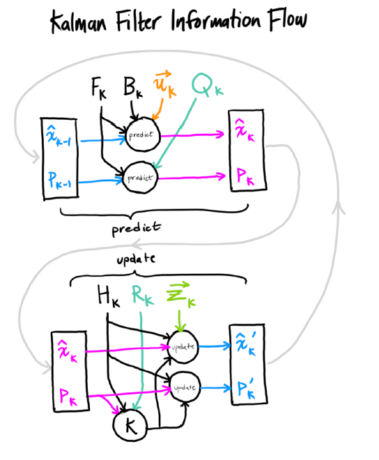
最终,可以卡尔曼滤波流程图如下:
参考:https://zhuanlan.zhihu.com/p/142044672
https://zhuanlan.zhihu.com/p/158751412
https://zhuanlan.zhihu.com/p/58675854
https://leijiezhang001.github.io/卡尔曼滤波详解/
https://zhuanlan.zhihu.com/p/166342719
3. 卡尔曼滤波用于目标跟踪
对于一个小车,我们采用卡尔曼滤波来估计其位置,在进行估计的时候,有几个变量要进行定义和初始化。这里定义了六个变量的初始值:状态向量,状态向量协方差矩阵,状态向量协方差矩阵的噪声矩阵,动态转移矩阵,映射矩阵,测量值得协方差矩阵(假设小车是匀速运动,所以没有使用控制矩阵和控制变量)
1. 初始状态向量(x):(8x1的矩阵)
其中对应含义和初始化值如下:
- (x,y)表示目标的中心点,a=w/h表示目标的宽高比,h表示目标的高度,初始化值为目标第一帧的位置
- v_x, v_y, v_a, v_h:表示对应变量随时间的变化率, 初始化值为0
2. 状态向量初始协方差矩阵(P):(8*8的矩阵, 这里如何设置,需要经验?)
3.状态向量协方差矩阵的噪声矩阵(Q):(8*8的矩阵, 这里如何设置,需要经验?)
4. 动态转移矩阵F:(8x8的矩阵)
5. 映射矩阵H:(4x8的矩阵)
6. 测量值的协方差矩阵(R):(4x4的矩阵, 这里如何设置,需要经验?)
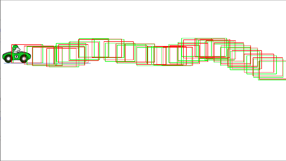
下面代码中,采用卡尔曼滤波,对小车的随机运动进行了估计,结果如图所示,绿色框表示小车的真实位置,红色框表示卡尔曼滤波的估计位置
# vim: expandtab:ts=4:sw=4
import numpy as np
import scipy.linalg
import cv2

"""
Table for the 0.95 quantile of the chi-square distribution with N degrees of
freedom (contains values for N=1, ..., 9). Taken from MATLAB/Octave's chi2inv
function and used as Mahalanobis gating threshold.
"""
chi2inv95 = {
    1: 3.8415,
    2: 5.9915,
    3: 7.8147,
    4: 9.4877,
    5: 11.070,
    6: 12.592,
    7: 14.067,
    8: 15.507,
    9: 16.919}


class KalmanFilter(object):
    """
    A simple Kalman filter for tracking bounding boxes in image space.

    The 8-dimensional state space

        x, y, a, h, vx, vy, va, vh

    contains the bounding box center position (x, y), aspect ratio a, height h,
    and their respective velocities.

    Object motion follows a constant velocity model. The bounding box location
    (x, y, a, h) is taken as direct observation of the state space (linear
    observation model).

    """

    def __init__(self):
        ndim, dt = 4, 1.

        # Create Kalman filter model matrices.
        self._motion_mat = np.eye(2 * ndim, 2 * ndim)  # 初始化动态转移矩阵, shape(8, 8)
        for i in range(ndim):
            self._motion_mat[i, ndim + i] = dt
        self._update_mat = np.eye(ndim, 2 * ndim)   # 初始化映射矩阵,shape(4, 8)

        # Motion and observation uncertainty are chosen relative to the current
        # state estimate. These weights control the amount of uncertainty in
        # the model. This is a bit hacky.
        self._std_weight_position = 1. / 20
        self._std_weight_velocity = 1. / 160

    def initiate(self, measurement):
        """Create track from unassociated measurement.

        Parameters
        ----------
        measurement : ndarray
            Bounding box coordinates (x, y, a, h) with center position (x, y),
            aspect ratio a, and height h.

        Returns
        -------
        (ndarray, ndarray)
            Returns the mean vector (8 dimensional) and covariance matrix (8x8
            dimensional) of the new track. Unobserved velocities are initialized
            to 0 mean.

        """
        mean_pos = measurement
        mean_vel = np.zeros_like(mean_pos)
        mean = np.r_[mean_pos, mean_vel]   # 状态向量,shape(1, 8)

        std = [
            2 * self._std_weight_position * measurement[3],
            2 * self._std_weight_position * measurement[3],
            1e-2,
            2 * self._std_weight_position * measurement[3],
            10 * self._std_weight_velocity * measurement[3],
            10 * self._std_weight_velocity * measurement[3],
            1e-5,
            10 * self._std_weight_velocity * measurement[3]]
        covariance = np.diag(np.square(std))    # 状态向量协方差矩阵, shape(8, 8)
        return mean, covariance

    def predict(self, mean, covariance):
        """Run Kalman filter prediction step.

        Parameters
        ----------
        mean : ndarray
            The 8 dimensional mean vector of the object state at the previous
            time step.
        covariance : ndarray
            The 8x8 dimensional covariance matrix of the object state at the
            previous time step.

        Returns
        -------
        (ndarray, ndarray)
            Returns the mean vector and covariance matrix of the predicted
            state. Unobserved velocities are initialized to 0 mean.

        """
        std_pos = [
            self._std_weight_position * mean[3],
            self._std_weight_position * mean[3],
            1e-2,
            self._std_weight_position * mean[3]]
        std_vel = [
            self._std_weight_velocity * mean[3],
            self._std_weight_velocity * mean[3],
            1e-5,
            self._std_weight_velocity * mean[3]]
        motion_cov = np.diag(np.square(np.r_[std_pos, std_vel]))

        mean = np.dot(self._motion_mat, mean)  # 动态转移矩阵*状态向量
        covariance = np.linalg.multi_dot((
            self._motion_mat, covariance, self._motion_mat.T)) + motion_cov   # 动态转移矩阵*状态向量协方差矩阵 + 噪声矩阵

        return mean, covariance

    def project(self, mean, covariance):
        """Project state distribution to measurement space.

        Parameters
        ----------
        mean : ndarray
            The state's mean vector (8 dimensional array).
        covariance : ndarray
            The state's covariance matrix (8x8 dimensional).

        Returns
        -------
        (ndarray, ndarray)
            Returns the projected mean and covariance matrix of the given state
            estimate.

        """
        std = [
            self._std_weight_position * mean[3],
            self._std_weight_position * mean[3],
            1e-1,
            self._std_weight_position * mean[3]]
        innovation_cov = np.diag(np.square(std))

        mean = np.dot(self._update_mat, mean)   # 映射矩阵*状态向量
        covariance = np.linalg.multi_dot((
            self._update_mat, covariance, self._update_mat.T))
        return mean, covariance + innovation_cov         # 映射矩阵*状态向量 + 噪声矩阵

    def update(self, mean, covariance, measurement):
        """Run Kalman filter correction step.

        Parameters
        ----------
        mean : ndarray
            The predicted state's mean vector (8 dimensional).
        covariance : ndarray
            The state's covariance matrix (8x8 dimensional).
        measurement : ndarray
            The 4 dimensional measurement vector (x, y, a, h), where (x, y)
            is the center position, a the aspect ratio, and h the height of the
            bounding box.

        Returns
        -------
        (ndarray, ndarray)
            Returns the measurement-corrected state distribution.

        """
        projected_mean, projected_cov = self.project(mean, covariance)

        chol_factor, lower = scipy.linalg.cho_factor(
            projected_cov, lower=True, check_finite=False)    # Cholesky分解
        kalman_gain = scipy.linalg.cho_solve(
            (chol_factor, lower), np.dot(covariance, self._update_mat.T).T,
            check_finite=False).T                             # 求解卡尔曼增益矩阵
        innovation = measurement - projected_mean

        new_mean = mean + np.dot(innovation, kalman_gain.T)    # 预测值和测量值融合后,新的状态向量
        new_covariance = covariance - np.linalg.multi_dot((
            kalman_gain, projected_cov, kalman_gain.T))        # 预测值和测量值融合后,新状态向量的协方差矩阵
        return new_mean, new_covariance

    def gating_distance(self, mean, covariance, measurements,
                        only_position=False):
        """Compute gating distance between state distribution and measurements.

        A suitable distance threshold can be obtained from `chi2inv95`. If
        `only_position` is False, the chi-square distribution has 4 degrees of
        freedom, otherwise 2.

        Parameters
        ----------
        mean : ndarray
            Mean vector over the state distribution (8 dimensional).
        covariance : ndarray
            Covariance of the state distribution (8x8 dimensional).
        measurements : ndarray
            An Nx4 dimensional matrix of N measurements, each in
            format (x, y, a, h) where (x, y) is the bounding box center
            position, a the aspect ratio, and h the height.
        only_position : Optional[bool]
            If True, distance computation is done with respect to the bounding
            box center position only.

        Returns
        -------
        ndarray
            Returns an array of length N, where the i-th element contains the
            squared Mahalanobis distance between (mean, covariance) and
            `measurements[i]`.

        """
        mean, covariance = self.project(mean, covariance)
        if only_position:
            mean, covariance = mean[:2], covariance[:2, :2]
            measurements = measurements[:, :2]

        cholesky_factor = np.linalg.cholesky(covariance)
        d = measurements - mean
        z = scipy.linalg.solve_triangular(
            cholesky_factor, d.T, lower=True, check_finite=False,
            overwrite_b=True)
        squared_maha = np.sum(z * z, axis=0)
        return squared_maha

if __name__ == "__main__":
    kf = KalmanFilter()
    img = cv2.imread("./car.png")
    m = np.array([108.5, 360.5, 1.618, 123])   # 小车的初始化测量值,分别表示小车的x_center, y_center, w/h, h
    mean_ini, covariance_ini = kf.initiate(m)  # 初始化卡尔曼的动态转移矩阵,映射矩阵


    for i in range(30):
        mean_pre, covariance_pre = kf.predict(mean_ini, covariance_ini)  # 预测状态变量
        dx = np.random.randint(0, 120)
        dy = np.random.randint(-30, 30)
        m = m + np.array([dx, dy, 0, 0])   # 随机向左,和上下移动
        cv2.rectangle(img, (int(m[0]-m[2]*m[3]/2), int(m[1]-m[3]/2)),
                      (int(m[0]+m[2]*m[3]/2), int(m[1]+m[3]/2)), (0, 255, 0), 2)  # 用绿色框,绘制小车移动后的真实位置

        mean_upd, covariance_upd = kf.update(mean_pre, covariance_pre, m+np.random.randn(4))   # 利用测量值,更新状态变量
        mean_ini = mean_upd
        covariance_ini = covariance_upd

        # 用红色框,绘制小车移动后的估计位置
        cv2.rectangle(img, (int(mean_ini[0] - mean_ini[2] * mean_ini[3] / 2), int(mean_ini[1] - mean_ini[3] / 2)),
                      (int(mean_ini[0] + mean_ini[2] * mean_ini[3] / 2), int(mean_ini[1] + mean_ini[3] / 2)), (0, 0, 255), 2)

        cv2.namedWindow("img", cv2.WINDOW_NORMAL)
        cv2.resizeWindow("img", 960, 540)
        cv2.imshow("img", img)
        cv2.waitKey(0)
        cv2.destroyAllWindows()