一:使用逻辑回归来识别手写数字(0-9)
(一)导入库,并且读取数据集
因为我们的数据集类型是.mat文件(是在matlab的本机格式),所以在使用python加载时,我们需要使用一个SciPy工具。
import numpy as np
import pandas as pd
import matplotlib as plt
from scipy.io import loadmat    #用于载入matlab文件

data = loadmat('ex3data1.mat')  #加载数据
print(data)
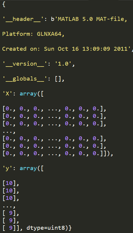
print(data['X'].shape)
print(data['y'].shape)
![]()
图像在martix X中表示为400维向量(其中有5000个数据)。400维“特征”是原始图像(20X20)图像中每个像素的灰度强度。
类标签在向量y中作为图像中数字的数字类。
第一个任务是将我们的逻辑函数实现修改为完全向量化(即没有for循环)。这是因为向量化代码除了简洁外,还能利用线性代数进行优化。
并且通常比迭代代码快得多。
(二)部分数据可视化(5000中,随机选取100个显示)
def displayData(X,example_width=None):  #显示20x20像素数据在一个格子里面
    if example_width is None:
        example_width = math.floor(math.sqrt(X.shape[1]))   #X.shape[1]=400
    print(X.shape)
    #计算行列
    m,n = X.shape   #返回的是我们随机选取的100行样本---(100,400)

    #获取图像高度
    example_height = math.ceil(n/example_width) #400/20 = 20

    # 计算需要展示的图片数量
    display_rows = math.floor(math.sqrt(m)) #10
    display_cols = math.ceil(m / display_rows)  #100/10=10

    fig,ax = plt.subplots(nrows=display_rows,ncols=display_cols,sharey=True,sharex=True,figsize=(12,12)) #https://blog.csdn.net/qq_39622065/article/details/82909421

    #拷贝图像到子区域进行展示
    for row in range(display_rows):
        for col in range(display_cols):
            ax[row,col].matshow(X[display_rows*row+col].reshape(example_width,example_height),cmap='gray') #希望将矩阵以图形方式显示https://www.cnblogs.com/shanger/articles/11872437.html

    plt.xticks([])  #用于设置每个小区域坐标轴刻度,设置为空,则不显示刻度
    plt.yticks([])

    plt.show()
plt.rcParams['figure.dpi'] = 200
data = loadmat('ex3data1.mat')  #加载数据
# print(data['X'].shape)
# print(data['y'].shape)
X = data.get('X')
y = data.get('y')
sample_idx = np.random.choice(np.arange(X.shape[0]),100)    #随机选取100个数(100个样本的序号)
# print(sample_idx)
samples = X[sample_idx,:]   #获取上面选取的索引对应的数据集
smaples_y = y[sample_idx,:] #可以知道我们选取的数字标签值
# print(smaples_y)
displayData(samples)  #进行展示

(三)sigmoid函数

def sigmoid(z): #实现sigmoid函数
    return 1/(1+np.exp(-z))
(四)正则化代价函数
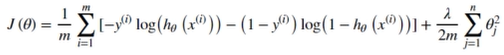
def regularized_cost(theta, X, y, learningRate=1):  #实现代价函数
    X = np.array(X)
    y = np.array(y)
    theta = np.array([theta])  #注意这一步:我们要对array类型进行矩阵运算,那么该数组必须是二维数组[[]]---如果我们这里直接使用np.array(theta),会导致代价函数求得准确率降低

    first = np.multiply(-y, np.log(sigmoid(X.dot(theta.T))))
    second = np.multiply((1 - y), np.log(1 - sigmoid(X.dot(theta.T))))
    reg = (learningRate/(2*len(X)))*np.sum(np.power(theta[1:theta.shape[0]],2))
    return np.sum(first - second) / (len(X)) + reg
(五)正则化梯度函数

def gradient(theta,X,y):    #实现求梯度
    return X.T@np.array((np.array(sigmoid(X @ theta)).reshape(-1, 1)-y))/len(X)

def regularized_gradient(theta,X,y,learningRate=1):
    theta_new = theta[1:]   #不加θ_0
    regularized_theta = (learningRate/len(X))*theta_new
    regularized_term = np.concatenate([np.array([0]),regularized_theta])    #前面加上0,是为了加给θ_0
    regularized_term = np.array(regularized_term).reshape(-1,1)
    return gradient(theta,X,y)+regularized_term
(六)构建分类器
我们已经定义了代价函数和梯度函数,现在应该进行分类器构建。对于这个任务,我们可能的类有10个,并且由于逻辑回归只能一次在两个类之间进行分类,我们需要多类分类的策略。
在本练习中,任务是实现一对全分类方法,其中具有K个不同类的标签就有K个分类器,每个分类器在“类别i和不是类别i”之间决定,我们将把分类器训练包含在一个函数中,该函数计算10个分类器中的每个分类器的最终权重,并将权重返回K*(n+1)数组,其中n是参数数量。
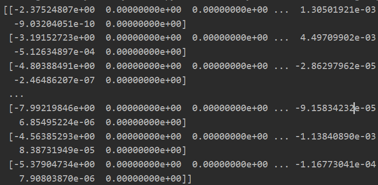
def one_to_all(X,y,num_labels,learning_rate):   #分类器构建  X训练集 y标签值 num_labels是构建的分类器数量(0-9标签值,则10个),learning_rate是入值
    rows = X.shape[0]
    cols = X.shape[1]

    #构建多维度θ值
    all_theta = np.zeros((num_labels,cols+1))   #这里我们需要添加θ_0,相应的我们要在X训练集中加入一列全为1的列向量

    #为X训练集添加一个全为1的列向量
    X = np.insert(X,0,values=np.ones(rows),axis=1)   #第二个参数是插入索引位置,第三个是插入数据,axis=1是列插入https://www.cnblogs.com/hellcat/p/7422005.html#_label2_9

    #开始进行参数拟合
    for i in range(1,num_labels+1):  #从1-10代替0-9,因为数据集的标签值是从1-10,print(np.unique(data['y']))可以知道
        theta = np.zeros(cols+1)    #初始化一个新的临时的θ值
        y_i = np.array([1 if label == i else 0 for label in y]) #进行二分类,对于对应的数设置为1,其他为0
        y_i = np.reshape(y_i,(rows,1))  #进行转置为列向量

        #使用高级优化算法进行参数迭代
        fmin = opt.minimize(fun=regularized_cost,x0=theta,args=(X, y_i),
                            method='TNC',jac=regularized_gradient)
        all_theta[i-1,:]=fmin.x #将1-10变为0-9

    return all_theta    #返回多维度θ值
plt.rcParams['figure.dpi'] = 200
data = loadmat('ex3data1.mat')  #加载数据
X = data.get('X')
y = data.get('y')

all_theta = one_to_all(X,y,10,1)
print(all_theta)
(七)对测试数据进行预测
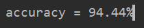
def predict_all(X,all_theta):   #输入测试数据X和参数θ    对测试数据进行预测
    #将我们的测试数据X前面插入一列零元素
    X = np.insert(X,0,1,axis=1) #X是(5000,401)   其中插入了一列
    #进行转置---可以直接合并到第3步
    all_theta = all_theta.T #all_theta原始是(10,401)转置后是(401,10)----10表示了每一个标签值(0-9)对应一个唯一的θ列

    #计算样本属于某一类的概率
    h = sigmoid(np.dot(X,all_theta))    #(5000,10)---5000个数据集对应10个标签值的的概率
    #找到每个测试数据中最大概率的数据---找到指定维度的最大值
    h_argmax = np.argmax(h,axis=1)  #返回沿轴axis最大值的索引。这里1表示行,0表示列。所以对于每一行数据,我们都会对应从10个标签值当中选取概率最大的值---预测数据对应的最可能对应的标签值
    #因为我们的数组是零索引的,所以我们想要为真正的标签+1
    h_argmax = h_argmax +1  #返回预测的数据集的标签

    return h_argmax
y_pred = predict_all(X,all_theta)
correct = [1 if a==b else 0 for (a,b) in zip(y_pred,y)] #重点:将预测值和原始值进行对比
accuracy = (sum(map(int,correct))/float(len(correct)))  #找到预测正确的数据/所有数据==百分比
print('accuracy = {0}%'.format(accuracy*100 ))
(八)全部代码


import math

import numpy as np
import pandas as pd
import matplotlib.pyplot as plt
from scipy.io import loadmat    #用于载入matlab文件
import scipy.optimize as opt

def displayData(X,example_width=None):  #显示20x20像素数据在一个格子里面
    if example_width is None:
        example_width = math.floor(math.sqrt(X.shape[1]))   #X.shape[1]=400
    print(X.shape)
    #计算行列
    m,n = X.shape   #返回的是我们随机选取的100行样本---(100,400)

    #获取图像高度
    example_height = math.ceil(n/example_width) #400/20 = 20

    # 计算需要展示的图片数量
    display_rows = math.floor(math.sqrt(m)) #10
    display_cols = math.ceil(m / display_rows)  #100/10=10

    fig,ax = plt.subplots(nrows=display_rows,ncols=display_cols,sharey=True,sharex=True,figsize=(12,12)) #https://blog.csdn.net/qq_39622065/article/details/82909421

    #拷贝图像到子区域进行展示
    for row in range(display_rows):
        for col in range(display_cols):
            ax[row,col].matshow(X[display_rows*row+col].reshape(example_width,example_height),cmap='gray') #希望将矩阵以图形方式显示https://www.cnblogs.com/shanger/articles/11872437.html

    plt.xticks([])  #用于设置每个小区域坐标轴刻度,设置为空,则不显示刻度
    plt.yticks([])

    plt.show()

def sigmoid(z):  # 实现sigmoid函数
    return 1 / (1 + np.exp(-z))

def regularized_cost(theta, X, y, learningRate=1):  #实现代价函数
    X = np.array(X)
    y = np.array(y)
    theta = np.array([theta])

    first = np.multiply(-y, np.log(sigmoid(X.dot(theta.T))))
    second = np.multiply((1 - y), np.log(1 - sigmoid(X.dot(theta.T))))
    reg = (learningRate/(2*len(X)))*np.sum(np.power(theta[1:theta.shape[0]],2))
    return np.sum(first - second) / (len(X)) + reg

def gradient(theta,X,y):    #实现求梯度
    return X.T@np.array((np.array(sigmoid(X @ theta)).reshape(-1, 1)-y))/len(X)

def regularized_gradient(theta,X,y,learningRate=1):
    theta_new = theta[1:]   #不加θ_0
    regularized_theta = (learningRate/len(X))*theta_new
    regularized_term = np.concatenate([np.array([0]),regularized_theta])    #前面加上0,是为了加给θ_0
    regularized_term = np.array(regularized_term).reshape(-1,1)
    return gradient(theta,X,y)+regularized_term

def one_to_all(X,y,num_labels,learning_rate):   #分类器构建  X训练集 y标签值 num_labels是构建的分类器数量(0-9标签值,则10个),learning_rate是入值
    rows = X.shape[0]
    cols = X.shape[1]

    #构建多维度θ值
    all_theta = np.zeros((num_labels,cols+1))   #这里我们需要添加θ_0,相应的我们要在X训练集中加入一列全为1的列向量

    #为X训练集添加一个全为1的列向量
    X = np.insert(X,0,values=np.ones(rows),axis=1)   #第二个参数是插入索引位置,第三个是插入数据,axis=1是列插入https://www.cnblogs.com/hellcat/p/7422005.html#_label2_9

    #开始进行参数拟合
    for i in range(1,num_labels+1):  #从1-10代替0-9,因为数据集的标签值是从1-10,print(np.unique(data['y']))可以知道
        theta = np.zeros(cols+1)    #初始化一个新的临时的θ值
        y_i = np.array([1 if label == i else 0 for label in y]) #进行二分类,对于对应的数设置为1,其他为0
        y_i = np.reshape(y_i,(rows,1))  #进行转置为列向量

        #使用高级优化算法进行参数迭代
        fmin = opt.minimize(fun=regularized_cost,x0=theta,args=(X, y_i),
                            method='TNC',jac=regularized_gradient)
        all_theta[i-1,:]=fmin.x #将1-10变为0-9

    return all_theta    #返回多维度θ值

def predict_all(X,all_theta):   #输入测试数据X和参数θ    对测试数据进行预测
    #将我们的测试数据X前面插入一列零元素
    X = np.insert(X,0,1,axis=1) #X是(5000,401)   其中插入了一列
    #进行转置---可以直接合并到第3步
    all_theta = all_theta.T #all_theta原始是(10,401)转置后是(401,10)----10表示了每一个标签值(0-9)对应一个唯一的θ列

    #计算样本属于某一类的概率
    h = sigmoid(np.dot(X,all_theta))    #(5000,10)---5000个数据集对应10个标签值的的概率
    #找到每个测试数据中最大概率的数据---找到指定维度的最大值
    h_argmax = np.argmax(h,axis=1)  #返回沿轴axis最大值的索引。这里1表示行,0表示列。所以对于每一行数据,我们都会对应从10个标签值当中选取概率最大的值---预测数据对应的最可能对应的标签值
    #因为我们的数组是零索引的,所以我们想要为真正的标签+1
    h_argmax = h_argmax +1  #返回预测的数据集的标签

    return h_argmax

plt.rcParams['figure.dpi'] = 200
data = loadmat('ex3data1.mat')  #加载数据
X = data.get('X')
y = data.get('y')

all_theta = one_to_all(X,y,10,1)

y_pred = predict_all(X,all_theta)
correct = [1 if a==b else 0 for (a,b) in zip(y_pred,y)] #重点:将预测值和原始值进行对比
accuracy = (sum(map(int,correct))/float(len(correct)))  #找到预测正确的数据/所有数据==百分比
print('accuracy = {0}%'.format(accuracy*100 ))

# #print(np.unique(data['y']))
# sample_idx = np.random.choice(np.arange(X.shape[0]),100)    #随机选取100个数(100个样本的序号)
# # print(sample_idx)
# samples = X[sample_idx,:]   #获取上面选取的索引对应的数据集
# smaples_y = y[sample_idx,:] #可以知道我们选取的数字标签值
# # print(smaples_y)
# displayData(samples)  #进行展示