Chapter 10 Image Segmentation 图像分割
10.2.7 Edge Linking and Boundary Detection 边缘连接和边界检测
Global processing using the Hough transform 使用霍夫变换的全局处理
-
一种检测像素集是否位于指定形状的曲线上的方法,一旦检测到,这些曲线就会形成边缘或感兴趣的区域边界。
-
霍夫变换:考虑 \(xy\) 平面上的一个点 \((x_i,y_i)\) 和形式为 \(y_i = ax_i + b\) 的一条直线。通过点的直线有无数条,且对a和b的不同值都满足方程。将该等式写为,考虑ab平面也称参数空间,将得到固定点的单一直线的方程。此外,第二个点在参数空间中也有一条与之相关联的直线,除非他们是平行的,否则这条直线会和相关联的直线相交于点。

- However,is that a(the slope of a line) approaches infinity as the line approaches the vertical direction.One way around this difficulty is to use the normal representation of a line:
- Each sinusoidal curve in Figure 10.32(b) represents the family of lines that pass through a particular point \((x_k,y_k)\) in the xy-plane. The intersection point \((\rho^{\prime},\theta^{\prime})\) corresponds to the line that passes through both \((x_i,y_i)\) and \((x_j,y_j)\)。 \((\rho^{\prime},\theta^{\prime})\) 对应于通过 \((x_i,y_i)\) 和 \((x_j,y_j)\)的直线。
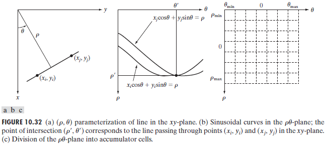
- The computational attractiveness of Hough transform arise from subdividing the $ \rho\theta $ parameter space into so-called accumulator cells(累加单元), as Fig.10.32(c)illustrates, where \((\rho\_{min},\rho\_{max})\) and \((\theta\_{min},\theta\_{max})\) are the expected ranges of the parameter values: \(-90^\circ \le \theta \le 90^\circ\) and \(-D \le \rho \le D\), where D is the maximum distance between opposite corners(对角线) in an image. The cell at coordinates \((i,j)\), with accumulator value \(A(i,j)\), corresponds to the square associated with parameter-space coordinates \((\rho_i,\theta_j)\). Initially, these cells are set to zero. Then, for every non-background point \((x_k,y_k)\) in the \(xy\)-plane, we let \(\theta\) equal each of the allowed subdivision values on the \(\theta\)-axis(令 \(\theta\) 等于 \(\theta\) 轴上每个允许的细分值) and solve for the corresponding \(\rho\) (解出相对应的 \(\rho\) ) using the equation \(\rho = x_kcos\theta + y_ksin\theta\). The resulting \(\rho\) values are then rounded off to the nearest allowed cell value along the \(\rho\) axis. If a choice of \(\theta_p\) results in solution \(\rho_q\), then we let \(A(p,q)=A(p,q)+1\). At the end of this procedure, a value of P in \(A(i,j)\) means that points in the \(xy\)-plane lie on the line \(xcos\theta_j + y sin\theta_j = \rho_i\). The number of subdivisions in the \(\rho\theta\)-plane determines the accuracy of the colinearity(共线性的精确性) of these points. It can be shown that the number of computations in the method just discussed is linear with respect to \(n\), the number of non-background points in the \(xy\)-plane.
-
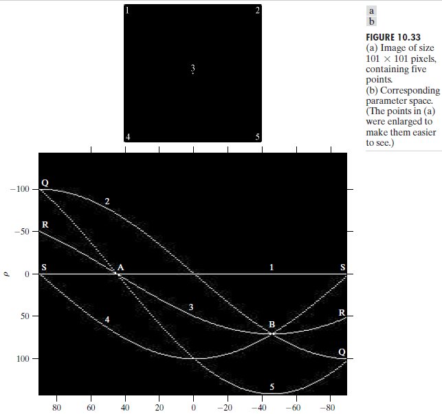
Example 图10.33(a)显示了一幅大小为101x101像素具有五个标记点的图像,图10.33(b)显示了将每个点映射到 \(\rho\theta\) 平面上的结果。其中A点和B点显示了霍夫变换的共线检测的性质。点A表示对应于xy图像平面内点1,3,5曲线的交点。点A的位置指出这三个点位于一条过原点且方向为45°的直线上。点B的位置指出点2,3,4位于方向为-45°且与原点的距离为\(\rho=71\)(即从原点到对角的对角线距离的一半)的直线上。最后,点Q、R、S表明霍夫变换展示了在参数空间左边缘和右边缘的一种反射邻接关系,这一性质是 \(\theta\) 和 \(\rho\) 在 \(\pm90°\) 边界改变符号的结果。
-
Although the focus thus far has been on straight lines, the Hough transform
is applicable to any function of the form \(g(v,c) = 0\) where v is a vector
of coordinates(坐标向量) and c is a vector of coefficients(系数向量). For example, points lying on the circle
can be detected by using the basic approach just discussed. The difference is
the presence of three parameters \((c_1,c_2,c_3)\), which results in a 3-D parameter
space with cube-like cells and accumulators of the form \(A(i,j,k)\). The
procedure is to increment \(c_1\) and \(c_2\) solve for \(c_3\) the that satisfies the equation above and update the accumulator cell associated with the triplet \((c_1,c_2,c_3)\)
10.3 Thresholding 阈值处理
10.3.3 Optimum Global Thresholding Using Otsu's Method 用OStu方法的最佳全局阈值处理
-
The approach discussed in this section, called Otsu’s method(大津阈值分割法) (Otsu [1979]), is an attractive alternative.The method is optimum in the sense that it maximizes
the between-class variance(最大化类间方差), a well-known measure used in statistical discriminant analysis. In addition to its optimality, Otsu’s method has the important property that it is based entirely on computations performed on the histogram of an image, an easily obtainable 1-D array. -
具体算法
- 设原始灰度图像灰度级为L,灰度级为i的像素点数为\(n_i\),则图像的全部像素数为
- 归一化直方图,则
- 按灰度级用阈值t划分为两类:\(C_0 = (0,1,...t)\) 和 \(C_1 = (t+1,t+2,...,L-1)\),因此,\(C_0\)和\(C_1\)类的出现概率及均值分别由下列各式给出
- 可以看出,对任何t值下式都能成立:
- C_0和C_1类的方差可由下式求得:
- 定义类内方差为:
- 类间方差为:
- 总体方差为:
10.3.7 Variable Thresholding 可变阈值处理
Using moving averages 使用移动平均
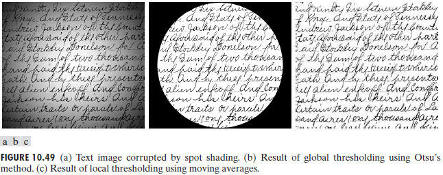
当需要处理的图像有非均匀分布的背景时,可以采用该方法
- Example
Interacitve Image Segmentation 交互式图像分割
- Step1-Feature Distribution Estimation
- Estimate the color distribution on scribbles
- Each pixel is assigned a probability to belong to F or B
- Step2-Weighted Distance Transform
- Weighted Geodesic Distance
- Computed in linear time
- Pixels are classified by comparing \(D_F(x)\) and \(D_B(x)\)
- Step3-Refine
- Automatically create a narrow band and new scribbles
- Band boundaries serve as "new scribbles"
Graph Cuts 图形分割技术 -Boykov and Jolly(2001)
- 详细内容参见该论文
Mumford-Shah Image Segmentation
Active Contours ("Snakes") 主动轮廓技术
- 可参考ipol.im网站上的算法:Chan-Vese Segmentation
- Demo - Otsu's Segmentation
I = imread('coins.png');
# 用大津阈值法计算最佳阈值
level = graythresh(I);
#用该阈值对图像进行分割
BW = im2bw(I,level);
#展示图像与直方图
figure,imshow(I),figure,imshow(BW),figure,imhist(I)