前言:
本次主要是练习下ICA模型,关于ICA模型的理论知识可以参考前面的博文:Deep learning:三十三(ICA模型)。本次实验的内容和步骤可以是参考UFLDL上的教程:Exercise:Independent Component Analysis。本次实验完成的内容和前面的很多练习类似,即学习STL-10数据库的ICA特征。当然了,这些数据已经是以patches的形式给出,共2w个patch,8*8大小的。
实验基础:
步骤分为下面几步:
- 设置网络的参数,其中的输入样本的维数为8*8*3=192。
- 对输入的样本集进行白化,比如说ZCA白化,但是一定要将其中的参数eplison设置为0。
- 完成ICA的代价函数和其导数公式。虽然在教程Exercise:Independent Component Analysis中给出的代价函数为:

(当然了,它还必须满足权值W是正交矩阵)。
但是在UFLDL前面的一个教程Deriving gradients using the backpropagation idea中给出的代价函数却为:
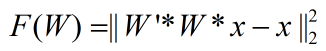
不过我感觉第2个代价函数要有道理些,并且在其教程中还给出了代价函数的偏导公式(这样实现时,可以偷懒不用推导了),只不过它给出的公式有一个小小的错误,我把正确的公式整理如下:

错误就是公式右边第一项最左边的那个应该是W,而不是它的转置W’,否则程序运行时是有矩阵维数不匹配的情况。
4. 最后就是对参数W进行迭代优化了,由于要使W满足正交性这一要求,所以不能直接像以前那样采用lbfgs算法,而是每次直接使用梯度下降法进行迭代,迭代完成后采用正交化步骤让W变成正交矩阵。只是此时文章中所说的学习率alpha是个动态变化的,是按照线性搜索来找到的。W正交性公式为:

5. 如果采用上面的代价函数和偏导公式时,用Ng给的code是跑不起来的,程序在线搜索的过程中会陷入死循环。(线搜索没有研究过,所以完全不懂)。最后在Deep Learning高质量交流群内网友”蜘蛛小侠”的提议下,将代价函数的W加一个特征稀疏性的约束,(注意此时的特征为Wx),然后把Ng的code中的迭代次数改大,比如5000,
其它程序不用更改,即可跑出结果来。
此时的代价函数为:

偏导为:

其中一定要考虑样本的个数m,否则即使通过了代价函数和其导数的验证,也不一定能通过W正交投影的验证。
实验结果:
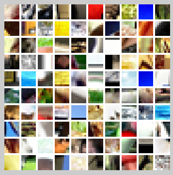
用于训练的样本显示如下:
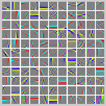
迭代20000次后的结果如下(因为电脑CUP不给力,跑了一天,当然了跑50000次结果会更完美,我就没时间验证了):
实验主要部分代码及注释:
ICAExercise.m:
%% CS294A/CS294W Independent Component Analysis (ICA) Exercise

%  Instructions
%  ------------
%
%  This file contains code that helps you get started on the
%  ICA exercise. In this exercise, you will need to modify
%  orthonormalICACost.m and a small part of this file, ICAExercise.m.

%%======================================================================
%% STEP 0: Initialization
%  Here we initialize some parameters used for the exercise.

numPatches = 20000;
numFeatures = 121;
imageChannels = 3;
patchDim = 8;
visibleSize = patchDim * patchDim * imageChannels;

outputDir = '.';
% 一般情况下都将L1规则项转换成平方加一个小系数然后开根号的形式,因为L1范数在0处不可微
epsilon = 1e-6; % L1-regularisation epsilon |Wx| ~ sqrt((Wx).^2 + epsilon)

%%======================================================================
%% STEP 1: Sample patches

patches = load('stlSampledPatches.mat');
patches = patches.patches(:, 1:numPatches);
displayColorNetwork(patches(:, 1:100));


%%======================================================================
%% STEP 2: ZCA whiten patches
%  In this step, we ZCA whiten the sampled patches. This is necessary for
%  orthonormal ICA to work.

patches = patches / 255;
meanPatch = mean(patches, 2);
patches = bsxfun(@minus, patches, meanPatch);

sigma = patches * patches';
[u, s, v] = svd(sigma);
ZCAWhite = u * diag(1 ./ sqrt(diag(s))) * u';
patches = ZCAWhite * patches;

%%======================================================================
%% STEP 3: ICA cost functions
%  Implement the cost function for orthornomal ICA (you don't have to
%  enforce the orthonormality constraint in the cost function)
%  in the function orthonormalICACost in orthonormalICACost.m.
%  Once you have implemented the function, check the gradient.

% Use less features and smaller patches for speed
% numFeatures = 5;
% patches = patches(1:3, 1:5);
% visibleSize = 3;
% numPatches = 5;
%
% weightMatrix = rand(numFeatures, visibleSize);
%
% [cost, grad] = orthonormalICACost(weightMatrix, visibleSize, numFeatures, patches, epsilon);
%
% numGrad = computeNumericalGradient( @(x) orthonormalICACost(x, visibleSize, numFeatures, patches, epsilon), weightMatrix(:) );
% % Uncomment to display the numeric and analytic gradients side-by-side
% % disp([numGrad grad]);
% diff = norm(numGrad-grad)/norm(numGrad+grad);
% fprintf('Orthonormal ICA difference: %g\n', diff);
% assert(diff < 1e-7, 'Difference too large. Check your analytic gradients.');
%
% fprintf('Congratulations! Your gradients seem okay.\n');


%%======================================================================
%% STEP 4: Optimization for orthonormal ICA
%  Optimize for the orthonormal ICA objective, enforcing the orthonormality
%  constraint. Code has been provided to do the gradient descent with a
%  backtracking line search using the orthonormalICACost function
%  (for more information about backtracking line search, you can read the
%  appendix of the exercise).
%
%  However, you will need to write code to enforce the orthonormality
%  constraint by projecting weightMatrix back into the space of matrices
%  satisfying WW^T  = I.
%
%  Once you are done, you can run the code. 10000 iterations of gradient
%  descent will take around 2 hours, and only a few bases will be
%  completely learned within 10000 iterations. This highlights one of the
%  weaknesses of orthonormal ICA - it is difficult to optimize for the
%  objective function while enforcing the orthonormality constraint -
%  convergence using gradient descent and projection is very slow.

weightMatrix = rand(numFeatures, visibleSize);%121*192
[cost, grad] = orthonormalICACost(weightMatrix(:), visibleSize, numFeatures, patches, epsilon);
fprintf('%11s%16s%10s\n','Iteration','Cost','t');
startTime = tic();

% Initialize some parameters for the backtracking line search
alpha = 0.5;
t = 0.02;
lastCost = 1e40;

% Do 10000 iterations of gradient descent
for iteration = 1:20000

    grad = reshape(grad, size(weightMatrix));
    newCost = Inf;
    linearDelta = sum(sum(grad .* grad));

    % Perform the backtracking line search
    while 1
        considerWeightMatrix = weightMatrix - alpha * grad;
        % -------------------- YOUR CODE HERE --------------------
        % Instructions:
        %   Write code to project considerWeightMatrix back into the space
        %   of matrices satisfying WW^T = I.
        %
        %   Once that is done, verify that your projection is correct by
        %   using the checking code below. After you have verified your
        %   code, comment out the checking code before running the
        %   optimization.

        % Project considerWeightMatrix such that it satisfies WW^T = I
%         error('Fill in the code for the projection here');
        considerWeightMatrix = (considerWeightMatrix*considerWeightMatrix')^(-0.5)*considerWeightMatrix;
        % Verify that the projection is correct
        temp = considerWeightMatrix * considerWeightMatrix';
        temp = temp - eye(numFeatures);
        assert(sum(temp(:).^2) < 1e-23, 'considerWeightMatrix does not satisfy WW^T = I. Check your projection again');
%         error('Projection seems okay. Comment out verification code before running optimization.');

        % -------------------- YOUR CODE HERE --------------------

        [newCost, newGrad] = orthonormalICACost(considerWeightMatrix(:), visibleSize, numFeatures, patches, epsilon);
        if newCost >= lastCost - alpha * t * linearDelta
            t = 0.9 * t;
        else
            break;
        end
    end

    lastCost = newCost;
    weightMatrix = considerWeightMatrix;

    fprintf('  %9d  %14.6f  %8.7g\n', iteration, newCost, t);

    t = 1.1 * t;

    cost = newCost;
    grad = newGrad;

    % Visualize the learned bases as we go along
    if mod(iteration, 10000) == 0
        duration = toc(startTime);
        % Visualize the learned bases over time in different figures so
        % we can get a feel for the slow rate of convergence
        figure(floor(iteration /  10000));
        displayColorNetwork(weightMatrix');
    end

end

% Visualize the learned bases
displayColorNetwork(weightMatrix');
orthonormalICACost.m:
function [cost, grad] = orthonormalICACost(theta, visibleSize, numFeatures, patches, epsilon)
%orthonormalICACost - compute the cost and gradients for orthonormal ICA
%                     (i.e. compute the cost ||Wx||_1 and its gradient)

    weightMatrix = reshape(theta, numFeatures, visibleSize);

    cost = 0;
    grad = zeros(numFeatures, visibleSize);

    % -------------------- YOUR CODE HERE --------------------
    % Instructions:
    %   Write code to compute the cost and gradient with respect to the
    %   weights given in weightMatrix.
    % -------------------- YOUR CODE HERE --------------------
    %% 法一:
    num_samples = size(patches,2);
%     cost = sum(sum((weightMatrix'*weightMatrix*patches-patches).^2))./num_samples+...
%             sum(sum(sqrt((weightMatrix*patches).^2+epsilon)))./num_samples;
%     grad = (2*weightMatrix*(weightMatrix'*weightMatrix*patches-patches)*patches'+...
%         2*weightMatrix*patches*(weightMatrix'*weightMatrix*patches-patches)')./num_samples+...
%         ((weightMatrix*patches./sqrt((weightMatrix*patches).^2+epsilon))*patches')./num_samples;
    cost = sum(sum((weightMatrix'*weightMatrix*patches-patches).^2))./num_samples+...
            sum(sum(sqrt((weightMatrix*patches).^2+epsilon)));
    grad = (2*weightMatrix*(weightMatrix'*weightMatrix*patches-patches)*patches'+...
        2*weightMatrix*patches*(weightMatrix'*weightMatrix*patches-patches)')./num_samples+...
        (weightMatrix*patches./sqrt((weightMatrix*patches).^2+epsilon))*patches';
    grad = grad(:);
end
参考资料: