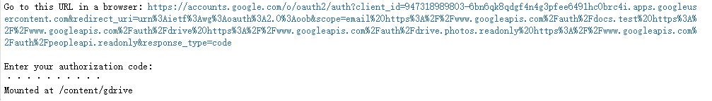
from google.colab import drive
drive.mount('/content/gdrive')
!mkdir '/content/gdrive/My Drive/dataset'
path = '/content/gdrive/My Drive/dataset/text8'
with  open(path) as ft_:
  full_text = ft_.read()
def  text_processing(ft8_text):
  '''
  替换掉标点符号
  '''
  ft8_text = ft8_text.lower()
  ft8_text = ft8_text.replace('.', '<period>')
  ft8_text = ft8_text.replace(',', '<comma>')
  ft8_text = ft8_text.replace('"', '<quotation>')
  ft8_text = ft8_text.replace(';', '<semicolon>')
  ft8_text = ft8_text.replace('!', '<exclamation>')
  ft8_text = ft8_text.replace('?', '<question>')
  ft8_text = ft8_text.replace('(', '<paren_l>')
  ft8_text = ft8_text.replace(')', '<paren_r>')
  ft8_text = ft8_text.replace('--', '<hyphen>')
  ft8_text = ft8_text.replace(':', '<colon>')
  ft8_text_tokens = ft8_text.split()
  return ft8_text_tokens

ft_tokens = text_processing(full_text)
import random
import collections
import math
import time
import re
import numpy as np

word_cnt = collections.Counter(ft_tokens)
shortlisted_words = [w for w in ft_tokens if word_cnt[w] > 7]
print(shortlisted_words[:15])

def  dict_creation(shortlisted_words):
  '''
  建立起单词和它出现频率之间的对应关系
  '''
  counts = collections.Counter(shortlisted_words)
  '''
  #将单词按出现次数由高到低排序,例如"the"出现最多就排第一位,它的序号为0,“an”次数第二多,序号
  对应为1,单词序号很重要,后面会用来建立单词的one-hot-vector,也就是把单词序号下标在向量中设置为1
  '''
  vocabulary = sorted(counts, key=counts.get, reverse=True)
  #将单词序号映射到单词
  rev_dictionary_ = {ii:word for ii, word in enumerate(vocabulary)}
  #将单词映射到序号,
  dictionary_ = {word: ii for ii, word in rev_dictionary_.items()}
  return dictionary_, rev_dictionary_

dictionary_, rev_dictionary_ = dict_creation(shortlisted_words)
words_cnt = [dictionary_[word] for word in shortlisted_words]
'''
根据负采样公式,把频率过低的单词过滤掉
'''
thresh = 0.00005
'''
建立单词序号与它出现次数的映射关系
'''
word_counts = collections.Counter(words_cnt)
total_count = len(words_cnt)
#建立单词与出现频率的对应关系
freqs = {word: count / total_count for word, count in word_counts.items()}
#根据负采样公式过滤单词
p_drop = { word: 1 - np.sqrt(thresh / freqs[word]) for word in word_counts}
train_words = [word for word in words_cnt if p_drop[word] < random.random()]
def  skipG_target_set_generation(batch_, batch_index, word_window):
  '''
  根据表12-1的方式构造网络训练数据
  '''
  random_num = np.random.randint(1, word_window + 1)
  #选择中心词左边窗口范围内的单词
  words_start = batch_index - random_num if (batch_index - random_num) > 0 else 0
  #选择中心词右边窗口范围内单词
  words_stop = batch_index + random_num
  window_target = set(batch_[words_start:batch_index] + batch_[batch_index+1 :
                                                               words_stop+1])
  return list(window_target)

def  skipG_batch_creation(short_words, batch_length, word_window):
  #将训练单词分批
  batch_cnt = len(short_words) // batch_length
  short_words = short_words[:batch_cnt * batch_length]

  for word_index in range(0, len(short_words), batch_length):
    #input_words是中心词
    #label_words 是中心词左右两边窗口范围内的单词
    input_words, label_words = [], []
    word_batch = short_words[word_index: word_index + batch_length]
    for index_ in range(len(word_batch)):
      batch_input = word_batch[index_]
      batch_label = skipG_target_set_generation(word_batch, index_, word_window)
      label_words.extend(batch_label)
      input_words.extend([batch_input] * len(batch_label))
      '''
      给定句子 ’the cat jump over the dog',窗口范围2,如果中心词是jump那么输出格式为
      input_words = [jump ,jump ,jump ,jump]
      label_words = [the, cat, over, the]
      '''
    yield input_words, label_words
import tensorflow as tf

tf_graph = tf.Graph()
with tf_graph.as_default():
  input_ = tf.placeholder(tf.int32, [None], name='input_')
  label_ = tf.placeholder(tf.int32, [None, None], name='label_')
  #构建中间二维向量
  word_embed = tf.Variable(tf.random_uniform((len(rev_dictionary_), 300), -1, 1))
  #计算one-hot-vector与中间向量乘机,其实就是把二维向量指定行选取出来
  embedding = tf.nn.embedding_lookup(word_embed, input_)

  vocabulary_size = len(rev_dictionary_)

  #添加中间层和输出层之间的链路参数,并使用正太分布对参数进行初始化
  sf_weights = tf.Variable(tf.truncated_normal((vocabulary_size, 300), stddev=0.1))
  sf_bias = tf.Variable(tf.zeros(vocabulary_size))
  '''
  使用梯度下降法训练参数,我们不训练所有参数而是随机选取第三层100个节点对应的链路参数进行修正,
  由于每个节点对应300个链路参数,因此总共修正的有(100+1)*300个参数
  '''
  loss_fn = tf.nn.sampled_softmax_loss(weights=sf_weights,
                                      biases=sf_bias,
                                      labels=label_,
                                      inputs=embedding,
                                      num_sampled=100,
                                      num_classes=vocabulary_size,
                                      )
  cost_fn = tf.reduce_mean(loss_fn)
  optim = tf.train.AdamOptimizer().minimize(cost_fn)
'''
使用余弦公式计算两个单词向量的距离,通过距离的大小展示单词含义是否相近
'''
with tf_graph.as_default():
  validation_cnt = 16
  validation_dict = 100

  #从编号为0到100的单词中随机选出8个
  validation_words = np.array(random.sample(range(validation_dict), validation_cnt//2))
  #再从编号为1000到1100的单词随机选出8个
  validation_words = np.append(validation_words, random.sample(range(1000,
                                                                    1000+validation_cnt),
                                                              validation_cnt//2))
  validation_data = tf.constant(validation_words, dtype=tf.int32)
  #先对单词向量做归一化处理
  normalization_embed = word_embed / (tf.sqrt(tf.reduce_sum(tf.square(word_embed),
                                                            1, keep_dims = True)))
  #将单词对应的向量挑选出来
  validation_embed = tf.nn.embedding_lookup(normalization_embed, validation_data)
  #计算两个向量内积,所得结果就是向量间距离
  word_similarity = tf.matmul(validation_embed, tf.transpose(normalization_embed))
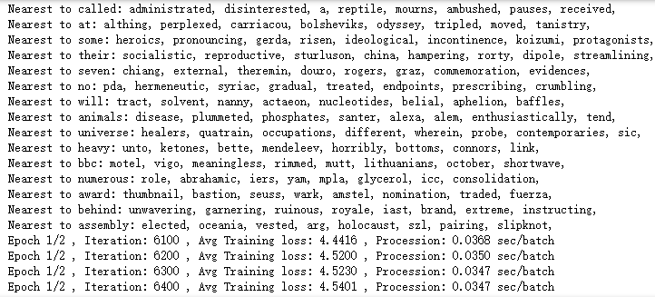
#循环训练10次,由于训练过程非常耗时,如果没有GPU,在训练时可以尝试把该值变小
epochs = 2
batch_length = 1000
word_window = 10

with tf_graph.as_default():
  saver = tf.train.Saver()

with tf.Session(graph = tf_graph) as sess:
  iteration = 1
  loss = 0
  sess.run(tf.global_variables_initializer())

  for e in range(1, epochs + 1):
    batches = skipG_batch_creation(train_words, batch_length, word_window)
    start = time.time()


    for x, y in batches:
      train_loss, _ = sess.run([cost_fn, optim], feed_dict={input_: x,
                                                           label_: np.array(y)[:, None]})
      loss += train_loss
      if iteration % 100 == 0:
        end = time.time()
        print("Epoch {}/{}".format(e, epochs), ", Iteration: {}".format(iteration),
             ", Avg Training loss: {:.4f}".format(loss/100),
             ", Procession: {:.4f} sec/batch".format((end - start) / 100))
        loss = 0
        start = time.time()
      #迭代训练2000次后计算一下单词相似度
      if iteration % 2000 == 0:
        similarity_ = word_similarity.eval()
        for i in range(validation_cnt):
          validated_words = rev_dictionary_[validation_words[i]]
          #根据计算距离,找出与当前单词距离最短的8个词
          top_k = 8
          nearest = (-similarity_[i, :]).argsort()[1: top_k+1]
          log = "Nearest to %s:" % validated_words
          for k in range(top_k):
            close_word =rev_dictionary_[nearest[k]]
            log = '%s %s,' % (log, close_word)
          print(log)

      iteration += 1

  path = '/content/gdrive/My Drive/skipGram_text8.ckpt'
  save_path = saver.save(sess, path)
  embed_mat = sess.run(normalization_embed)
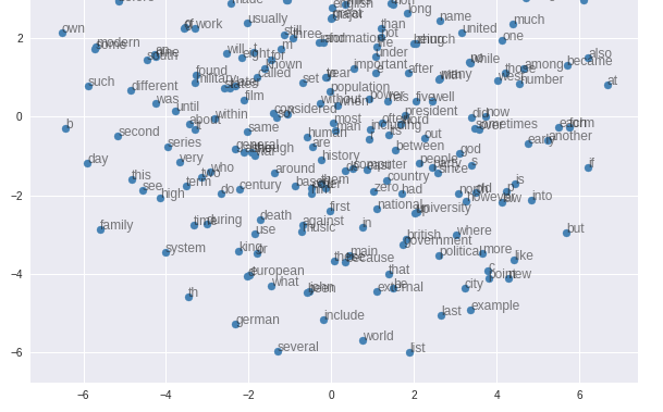
import matplotlib.pyplot as plt
from sklearn.manifold import TSNE

with tf.Session(graph=tf_graph) as sess:
  path = '/content/gdrive/My Drive/skipGram_text8_epoch10.ckpt'
  saver = tf.train.import_meta_graph(path + '.meta')
  #将训练后存储成文件的网络参数重新加载
  saver.restore(sess, path)
  sess.run(tf.global_variables_initializer())
  embed_mat = sess.run(word_embed)
  #选取250个单词向量在二维平面上展示
  word_graph = 250
  tsne = TSNE()
  word_embedding = tsne.fit_transform(embed_mat[:word_graph,:])
  fig, ax = plt.subplots(figsize=(10, 10))
  for idx in range(word_graph):
    plt.scatter(*word_embedding[idx, :], color='steelblue')
    plt.annotate(rev_dictionary_[idx], (word_embedding[idx, 0], word_embedding[idx, 1]), alpha=0.6)