机器学习笔记（五）过拟合问题及正则化

一、 过拟合问题

1. 引入

线性回归当中：

 

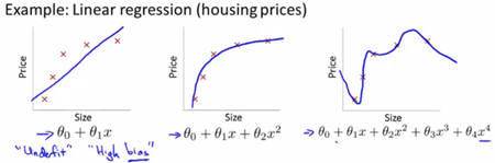
假设我们拿出房屋面积与房价的数据集，随着面积的增大，房价曲线趋于平缓。第一个模型不能很好地拟合，具有高偏差（欠拟合）。我们加入二次项后曲线可以较好的拟合，用第三个模型去拟合时，它通过了所有的数据点，但它是一条扭曲的线条，不停上下波动，我们并不认为它是一个预测房价的好模型。这个现象我们称为过度拟合。

（概括：过拟合现象常在变量过多的时候出现，能非常好的拟合训练数据，但无法泛化到新样本中。）

同样地，Logistic回归当中：

解决过拟合问题：

1)  减少特征数量

2)  正则化方法

二、正则化

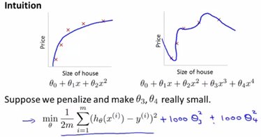
上图第二个模型不是一个好的拟合模型，现在我们在三次项和四次项上面加上惩罚项（penalize）如1000，我们要最小化这个新函数，就是 和 要尽可能小，他们会趋近于0，最后我们拟合得到的函数实际上是一个二次函数。总体来说我们在一些项上面加上惩罚项就相当于简化这个函数，使之更不容易出现过拟合的问题。

在实际问题中，如一个问题有100个参数，我们不知道该选择哪个它和标签相关度较低，此时我们修改代价函数来缩小所有的参数。

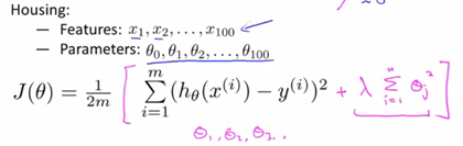
在代价函数中添加一个额外的正则化项，来缩小每个参数的值。

1.  线性回归的正则化

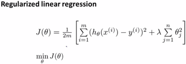
在usual linear regression基础上加上一个额外的正则化项，其中是正则化参数，我们不需要对一项进行正则化。

梯度下降法：

我们将与其他参数的更新过程分开，在此基础上求偏导数，这样就可以对正则化代价函数使用梯度下降的方法进行最小化。

课堂记录：

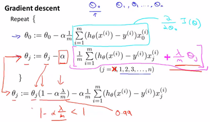
其中由于学习率很小，m很大，是一个略小于1的数，举例可能是0.99，这一项乘上相当于每次更新将向0方向缩小一点点。

正规方程法：

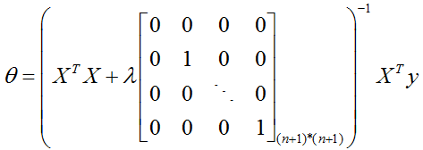这就是正则化后的正规方程法公式。

PS：关于矩阵不可逆问题，如果正则化参数我们就可以保证括号中的矩阵一定是可逆的，因为正则化正好可以解决一些不可逆的问题。

2.  Logistic回归的正则化

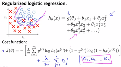
加上一个额外的正则化项之后，即使我们有很多的特征和参数，也可以得到一个较好的拟合模型，避免过拟合现象。

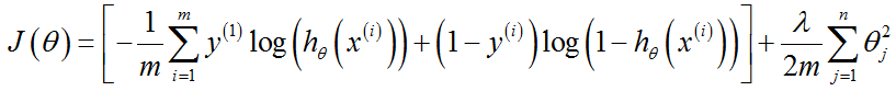
代价函数和梯度：

 

 代价函数增加了一个正则化项，梯度也随之相应改变。

实现部分

下面是在上一篇笔记《Logistic回归模型实现》costFunction.m代码的基础啊上我们修改过后，正则化后的costFunctionReg.m

function [J, grad] = costFunctionReg(theta, X, y, lambda)
%COSTFUNCTIONREG Compute cost and gradient for logistic regression with regularization
m = length(y); % number of training examples

J = 0;
grad = zeros(size(theta));
% =============================================================
J = 1/m * (-y' * log(sigmoid(X*theta)) - (1 - y') * log(1 - sigmoid(X * theta))) + lambda/2/m*sum(theta(2:end).^2); 
grad(1,:) = 1/m * (X(:, 1)' * (sigmoid(X*theta) - y));
grad(2:size(theta), :) = 1/m * (X(:, 2:size(theta))' * (sigmoid(X*theta) - y))... 
    + lambda/m*theta(2:size(theta), :);

end

下面是lambda取值为【0,1,10,100】时的拟合结果，从结果可以看出，lambda = 0时，可能存在过拟合现象，lambda = 1/10时，获得较好模型。

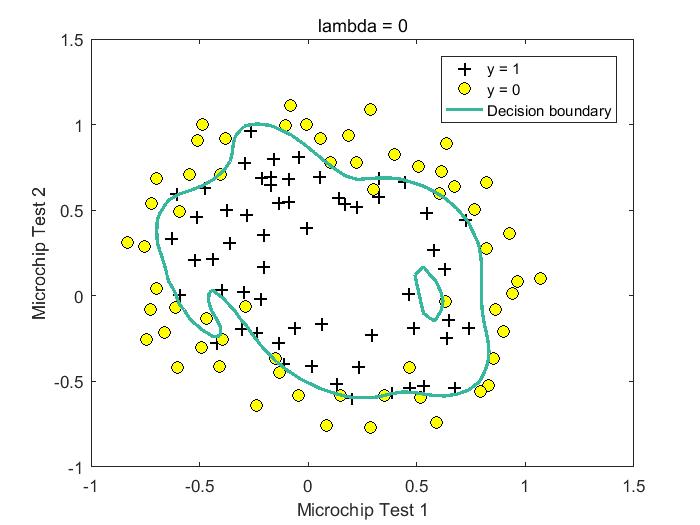
%lambda = 0
Train Accuracy: 87.288136

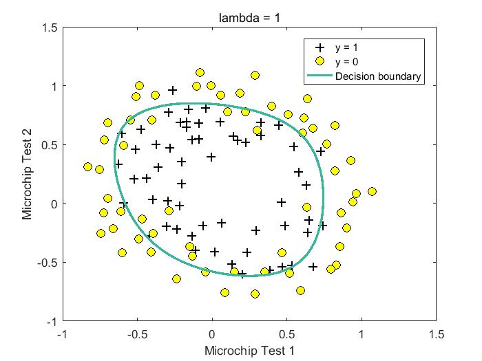
%lambda = 1
Train Accuracy: 83.050847
Expected accuracy (with lambda = 1): 83.1 (approx)

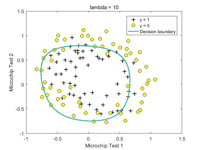
%lambda = 10
Train Accuracy: 83.050847

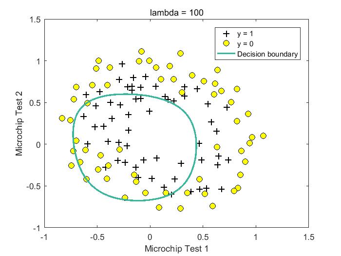
%lambda = 100
Train Accuracy: 61.016949

过程代码：

%% Machine Learning Online Class - Exercise 2: Logistic Regression
%% Initialization
clear ; close all; clc

%% Load Data
%  The first two columns contains the X values and the third column
%  contains the label (y).

data = load('ex2data2.txt');
X = data(:, [1, 2]); y = data(:, 3);

plotData(X, y);
hold on;
xlabel('Microchip Test 1')
ylabel('Microchip Test 2')

% Specified in plot order
legend('y = 1', 'y = 0')
hold off;


%% =========== Part 1: Regularized Logistic Regression ============
% Add Polynomial Features
% Note that mapFeature also adds a column of ones for us, so the intercept
% term is handled
X = mapFeature(X(:,1), X(:,2));

% Initialize fitting parameters
initial_theta = zeros(size(X, 2), 1);

% Set regularization parameter lambda to 1
lambda = 100;

% Compute and display initial cost and gradient for regularized logistic
% regression
[cost, grad] = costFunctionReg(initial_theta, X, y, lambda);

fprintf('Cost at initial theta (zeros): %f
', cost);
fprintf('Expected cost (approx): 0.693
');
fprintf('Gradient at initial theta (zeros) - first five values only:
');
fprintf(' %f 
', grad(1:5));
fprintf('Expected gradients (approx) - first five values only:
');
fprintf(' 0.0085
 0.0188
 0.0001
 0.0503
 0.0115
');

fprintf('
Program paused. Press enter to continue.
');
pause;

% Compute and display cost and gradient
% with all-ones theta and lambda = 10
test_theta = ones(size(X,2),1);
[cost, grad] = costFunctionReg(test_theta, X, y, 10);

fprintf('
Cost at test theta (with lambda = 10): %f
', cost);
fprintf('Expected cost (approx): 3.16
');
fprintf('Gradient at test theta - first five values only:
');
fprintf(' %f 
', grad(1:5));
fprintf('Expected gradients (approx) - first five values only:
');
fprintf(' 0.3460
 0.1614
 0.1948
 0.2269
 0.0922
');

fprintf('
Program paused. Press enter to continue.
');
pause;

%% ============= Part 2: Regularization and Accuracies =============
%  Optional Exercise:
%  In this part, you will get to try different values of lambda and
%  see how regularization affects the decision coundart
%
%  Try the following values of lambda (0, 1, 10, 100).
%
%  How does the decision boundary change when you vary lambda? How does
%  the training set accuracy vary?
% Initialize fitting parameters 
initial_theta = zeros(size(X, 2), 1); 
% Set regularization parameter lambda to 1 (you should vary this) 
lambda = 0; 
% Set Options 
options = optimset('GradObj', 'on', 'MaxIter', 400); 
% Optimize 
[theta, J, exit_flag] = ... 
    fminunc(@(t)(costFunctionReg(t, X, y, lambda)), initial_theta, options); 
% Plot Boundary 
plotDecisionBoundary(theta, X, y); 
hold on; 
title(sprintf('lambda = %g', lambda)) 
% Labels and Legend 
xlabel('Microchip Test 1') 
ylabel('Microchip Test 2') 
legend('y = 1', 'y = 0', 'Decision boundary') 
hold off; 
% Compute accuracy on our training set 
p = predict(theta, X); 
fprintf('Train Accuracy: %f
', mean(double(p == y)) * 100); 
fprintf('Expected accuracy (with lambda = 0): (approx)
');