一、多元分类
1.1 数据集
本次实现的是手写数字的识别,数据集中有5000个样本,其中每个样本是20*20像素的一张图片,每个像素都用一个点数来表示,该点数表示这个位置的灰度,将20*20的像素网络展开为400维向量,而训练集中的5000*400的矩阵,每一行就代表了一个手写数字图像的灰度值。
训练集的第二部分是5000维向量y,包含训练集的标签,为了与没有0索引的MATLAB索引兼容,我们将数字零映射到10,因此, 0“数字被标记为 10”,而数字 1“至 9”则按照其自然顺序被标记为 1“至 9”。
1.2 可视化数据
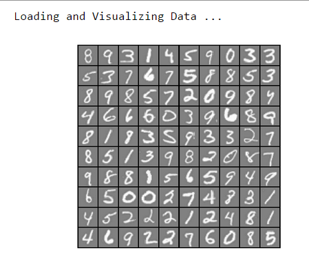
可视化数据的代码已经完成,运行可以看到随机从数据集中挑选出来的100个数字
数据可视化函数:
function [h, display_array] = displayData(X, example_width)
%DISPLAYDATA Display 2D data in a nice grid
%   [h, display_array] = DISPLAYDATA(X, example_width) displays 2D data
%   stored in X in a nice grid. It returns the figure handle h and the
%   displayed array if requested.

% Set example_width automatically if not passed in
if ~exist('example_width', 'var') || isempty(example_width)
    example_width = round(sqrt(size(X, 2)));
end

% Gray Image
colormap(gray);

% Compute rows, cols
[m n] = size(X);
example_height = (n / example_width);

% Compute number of items to display
display_rows = floor(sqrt(m));
display_cols = ceil(m / display_rows);

% Between images padding
pad = 1;

% Setup blank display
display_array = - ones(pad + display_rows * (example_height + pad), ...
                       pad + display_cols * (example_width + pad));

% Copy each example into a patch on the display array
curr_ex = 1;
for j = 1:display_rows
    for i = 1:display_cols
        if curr_ex > m,
            break;
        end
        % Copy the patch

        % Get the max value of the patch
        max_val = max(abs(X(curr_ex, :)));
        display_array(pad + (j - 1) * (example_height + pad) + (1:example_height), ...
                      pad + (i - 1) * (example_width + pad) + (1:example_width)) = ...
                        reshape(X(curr_ex, :), example_height, example_width) / max_val;
        curr_ex = curr_ex + 1;
    end
    if curr_ex > m,
        break;
    end
end

% Display Image
h = imagesc(display_array, [-1 1]);

% Do not show axis
axis image off

drawnow;

end
调用显示函数:
% Load Training Data
fprintf('Loading and Visualizing Data ...
')

load('ex3data1.mat'); % training data stored in arrays X, y
m = size(X, 1);
% Randomly select 100 data points to display
rand_indices = randperm(m);
sel = X(rand_indices(1:100), :);

displayData(sel);

fprintf('Program paused. Press enter to continue.
');
pause;
运行结果:
1.3 向量化logistic回归
1.3.1 向量化代价函数
从向量化代价函数开始,logistic回归的代价函数是: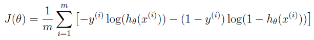 ,为了求和,我们要计算每个样本i的
![]() ,而
,而![]() ,
,![]() 是sigmoid函数。
是sigmoid函数。
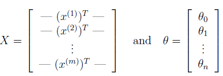
我们定义X和θ为:
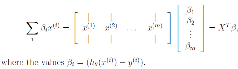
然后计算矩阵乘法Xθ,等于
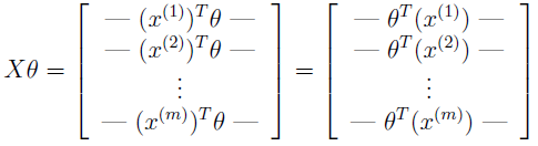 (注意这里运用了向量运算的法则
![]() )
)
这使得我们计算所有样本的![]() 时只要使用一行代码即可。
时只要使用一行代码即可。
1.3.2 向量化梯度
回顾一下非正则化逻辑回归成本函数的梯度是一个向量,其中第J个元素定义为![]() ,我们写出所有
,我们写出所有![]() 的偏导数:
的偏导数:
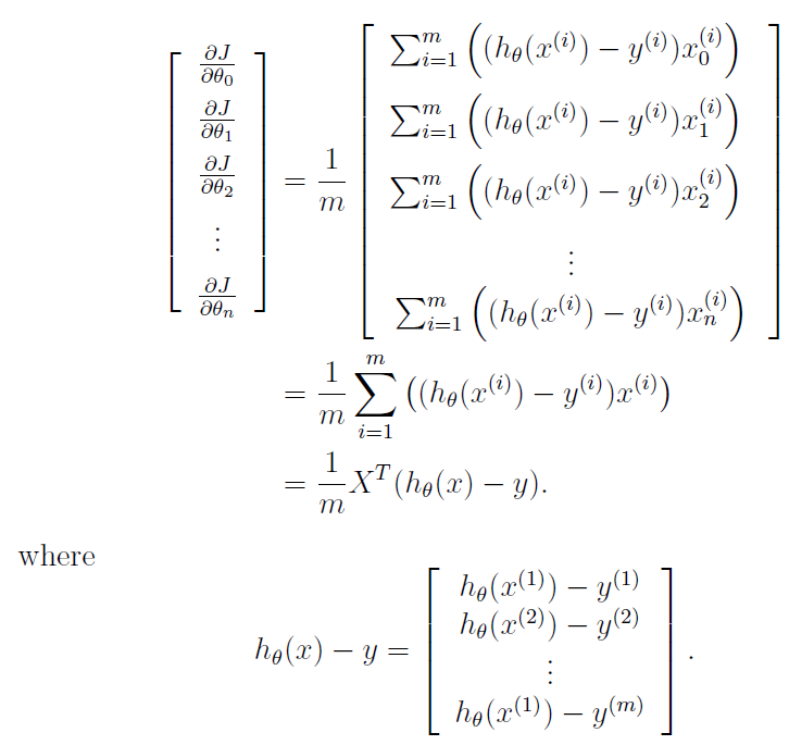
理解一下上述推导中的最后一步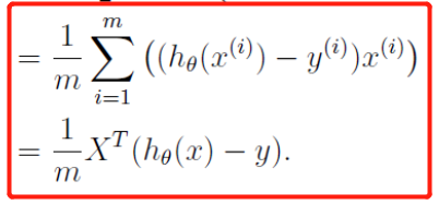 ,我们定义
,我们定义![]() ,于是可以得到:
,于是可以得到:
1.3.3 向量化正则化的逻辑回归
完成logistic回归的向量化后,这时候往代价函数中增加正则化项,之前学过,正则化的logistic回归的代价函数为:
![]() (注意θ0不需要正则化,因为它是用来控制偏置项的)
(注意θ0不需要正则化,因为它是用来控制偏置项的)
正则化的logistic回归的代价函数偏导数定义为:
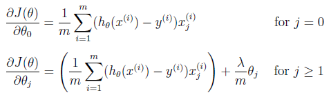
完成lrcostfunction.m中的代码,要使用元素乘法和求和函数sum:
function [J, grad] = lrCostFunction(theta, X, y, lambda)
%LRCOSTFUNCTION Compute cost and gradient for logistic regression with
%regularization
%   J = LRCOSTFUNCTION(theta, X, y, lambda) computes the cost of using
%   theta as the parameter for regularized logistic regression and the
%   gradient of the cost w.r.t. to the parameters.

% Initialize some useful values
m = length(y); % number of training examples

% You need to return the following variables correctly
J = 0;
grad = zeros(size(theta));

% ====================== YOUR CODE HERE ======================
% Instructions: Compute the cost of a particular choice of theta.
%               You should set J to the cost.
%               Compute the partial derivatives and set grad to the partial
%               derivatives of the cost w.r.t. each parameter in theta
%
% Hint: The computation of the cost function and gradients can be
%       efficiently vectorized. For example, consider the computation
%
%           sigmoid(X * theta)
%
%       Each row of the resulting matrix will contain the value of the
%       prediction for that example. You can make use of this to vectorize
%       the cost function and gradient computations.
%
% Hint: When computing the gradient of the regularized cost function,
%       there're many possible vectorized solutions, but one solution
%       looks like:
%           grad = (逻辑回归未正则化的梯度)
%           temp = theta;
%           temp(1) = 0;   % because we don't add anything for j = 0
%           grad = grad + YOUR_CODE_HERE (使用temp变量)

hy = sigmoid(X*theta);
J = sum(-y.*log(hy) - (1-y).*log(1-hy))/m;  % 计算未正则化的代价函数
diff = hy - y;
grad = X'*diff/m; % 未正则化的梯度
J = J + sum(theta(2:end).^2)*lambda/(2*m);  % 正则化后的代价函数(theta从第二个开始)
temp = theta;
temp(1) = 0;
grad = grad + temp*(lambda/m);

% =============================================================

grad = grad(:);

end
运行得到的结果:

1.4 一对多分类
训练多个正则逻辑回归分类器实现一对多分类,在给出的手写数字数据集中,类别K=10,而我们编写的代码应该适用于任何K值
tip:MATLAB中,向量a(m*1)和标量b进行a==b的运算,将会得到一个和a相同size的向量,代码示例如下:
>> a =1:10
a =
     1     2     3     4     5     6     7     8     9    10
>> b=3
b =
     3
>> a==b
ans =
  1×10 logical 数组
   0   0   1   0   0   0   0   0   0   0
完成oneVSall.m中的代码:
function [all_theta] = oneVsAll(X, y, num_labels, lambda)
%ONEVSALL trains multiple logistic regression classifiers and returns all
%the classifiers in a matrix all_theta, where the i-th row of all_theta
%corresponds to the classifier for label i
% ONEVSALL训练多个逻辑回归分类器,并以矩阵all_theta返回所有分类器,其中all_theta的第i行对应于标签i的分类器
%   [all_theta] = ONEVSALL(X, y, num_labels, lambda) trains num_labels
%   logistic regression classifiers and returns each of these classifiers
%   in a matrix all_theta, where the i-th row of all_theta corresponds
%   to the classifier for label i

% Some useful variables
m = size(X, 1); % 返回X矩阵的第一个维度(行)数
n = size(X, 2); % 返回X矩阵的第二个维度(列)数

% You need to return the following variables correctly
all_theta = zeros(num_labels, n + 1);

% Add ones to the X data matrix 给X矩阵加上一列1
X = [ones(m, 1) X];

% ====================== YOUR CODE HERE ======================
% Instructions: You should complete the following code to train num_labels
%               logistic regression classifiers with regularization
%               parameter lambda.
%
% Hint: theta(:) will return a column vector.
%
% Hint: You can use y == c to obtain a vector of 1's and 0's that tell you
%       whether the ground truth is true/false for this class.
%
% Note: For this assignment, we recommend using fmincg to optimize the cost
%       function. It is okay to use a for-loop (for c = 1:num_labels) to
%       loop over the different classes.
%
%       fmincg works similarly to fminunc, but is more efficient when we
%       are dealing with large number of parameters.
% 在这里我们使用fmincg函数来优化代价函数,fmincg和fminunc基本相同,但是前者处理大量数据效率更高
% Example Code for fmincg:
%
%     % Set Initial theta
%     initial_theta = zeros(n + 1, 1);
%
%     % Set options for fminunc
%     options = optimset('GradObj', 'on', 'MaxIter', 50);
%
%     % Run fmincg to obtain the optimal theta
%     % This function will return theta and the cost
%     [theta] = ...
%         fmincg (@(t)(lrCostFunction(t, X, (y == c), lambda)), ...
%                 initial_theta, options);
%
% options = optimset('GradObj', 'on', 'MaxIter', 50);
%
% for c = 1:num_labels
% initial_theta = zeros(n+1, 1);
% all_theta(c,:) = fmincg(@(t)(lrCostFunction(t, X, (y==c), lambda)), initial_theta, options);
% end
for c=1:num_labels
initial_theta = zeros(n+1,1);
options = optimset('GradObj', 'on', 'MaxIter', 50);
%调用fmincg库函数求出所有分类器的θ向量
[theta] = ...
fmincg (@(t)(lrCostFunction(t, X, (y == c), lambda)), ...
initial_theta, options);
%将每个θ放入all_theta的每一行中
all_theta(c,:) = theta';
% =========================================================================

end
运行结果:
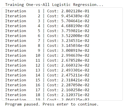
num_labels 为分类器个数,共10个,每个分类器(模型)用来识别10个数字中的某一个。
我们一共有5000个样本,每个样本有400个特征变量,因此:模型参数θ向量有401个元素。
initial_theta = zeros(n+1,1); % 模型参数θ的初始值(n == 400)
all_theta是一个10*401的矩阵,每一行存储着一个分类器(模型)的模型参数θ向量,执行上面for循环,就调用fmincg库函数求出了所有模型的参数θ向量了。
1.4.1 一对多预测
训练完分类器以后,可以使用它来预测图像代表的数字,对于每个输入,使用经过训练的逻辑回归分类器来计算属于每个类别的概率,最后输出概率最高的一个作为预测的结果。
完成predictOneVsAll.m中的代码:
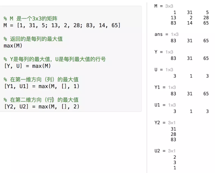
function p = predictOneVsAll(all_theta, X)
m = size(X, 1);
num_labels = size(all_theta, 1); % 定义num_labels为all_theta矩阵的行数(本例中为10)

% You need to return the following variables correctly
p = zeros(size(X, 1), 1);

% Add ones to the X data matrix
X = [ones(m, 1) X];

[x,p] = max(sigmoid(X*all_theta'),[],2); %返回的p为预测函数中最大值的行号

end
调用函数,看一下预测准确率:
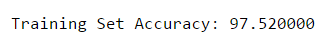
pred = predictOneVsAll(all_theta, X);

fprintf('
Training Set Accuracy: %f
', mean(double(pred == y)) * 100);
输出结果:

2. 神经网络
2.1 模型表示
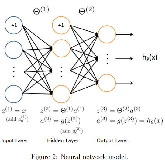
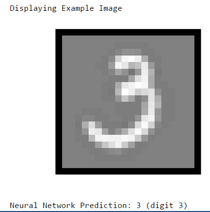
本神经网络中,参数已经训练完并给出,只需要加载到theta_1和theta_2中,该神经网络在第二层有25个单位,在输出层有10个单位,完成predict.m中的代码
function p = predict(Theta1, Theta2, X)

% Useful values
m = size(X, 1);
num_labels = size(Theta2, 1);

% You need to return the following variables correctly
p = zeros(size(X, 1), 1);

a1 = [ones(m, 1) X]; % 输入层 a1是X前加一列
a2 = [ones(m,1) sigmoid(a1 * Theta1')]; % 隐藏层 a2是用theta_1计算出的第二层
[x, p] = max(sigmoid(a2 * Theta2'), [], 2); % 输出层

end
预测结果: