cell 1 显示设置初始化
 1 # A bit of setup
 2
 3 import numpy as np
 4 import matplotlib.pyplot as plt
 5
 6 from cs231n.classifiers.neural_net import TwoLayerNet
 7
 8 %matplotlib inline
 9 plt.rcParams['figure.figsize'] = (10.0, 8.0) # set default size of plots
10 plt.rcParams['image.interpolation'] = 'nearest'
11 plt.rcParams['image.cmap'] = 'gray'
12
13 # for auto-reloading external modules
14 # see http://stackoverflow.com/questions/1907993/autoreload-of-modules-in-ipython
15 %load_ext autoreload
16 %autoreload 2
17
18 def rel_error(x, y):
19   """ returns relative error """
20   return np.max(np.abs(x - y) / (np.maximum(1e-8, np.abs(x) + np.abs(y))))
cell 2 网络模型与数据初始化函数
 1 # Create a small net and some toy data to check your implementations.
 2 # Note that we set the random seed for repeatable experiments.
 3
 4 input_size = 4
 5 hidden_size = 10
 6 num_classes = 3
 7 num_inputs = 5
 8
 9 def init_toy_model():
10   np.random.seed(0)
11   return TwoLayerNet(input_size, hidden_size, num_classes, std=1e-1)
12
13 def init_toy_data():
14   np.random.seed(1)
15   X = 10 * np.random.randn(num_inputs, input_size)
16   y = np.array([0, 1, 2, 2, 1])
17   return X, y
18
19 net = init_toy_model()
20 X, y = init_toy_data()
通过末尾的调用,生成了NN类,并生成了测试数据。
类的初始化代码(cs231n/classifiers/neural_net.py):
 1   def __init__(self, input_size, hidden_size, output_size, std=1e-4):
 2     """
 3     Initialize the model. Weights are initialized to small random values and
 4     biases are initialized to zero. Weights and biases are stored in the
 5     variable self.params, which is a dictionary with the following keys:
 6
 7     W1: First layer weights; has shape (D, H)
 8     b1: First layer biases; has shape (H,)
 9     W2: Second layer weights; has shape (H, C)
10     b2: Second layer biases; has shape (C,)
11
12     Inputs:
13     - input_size: The dimension D of the input data.
14     - hidden_size: The number of neurons H in the hidden layer.
15     - output_size: The number of classes C.
16     """
17     self.params = {}
18     self.params['W1'] = std * np.random.randn(input_size, hidden_size)
19     self.params['b1'] = np.zeros(hidden_size)
20     self.params['W2'] = std * np.random.randn(hidden_size, output_size)
21     self.params['b2'] = np.zeros(output_size)
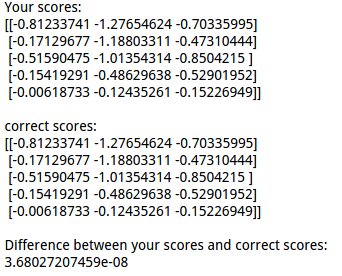
cell 3 前向传播计算loss,得到的结果与参考结果对比,证明模型的正确性:
 1 scores = net.loss(X)
 2 print 'Your scores:'
 3 print scores
 4 print
 5 print 'correct scores:'
 6 correct_scores = np.asarray([
 7   [-0.81233741, -1.27654624, -0.70335995],
 8   [-0.17129677, -1.18803311, -0.47310444],
 9   [-0.51590475, -1.01354314, -0.8504215 ],
10   [-0.15419291, -0.48629638, -0.52901952],
11   [-0.00618733, -0.12435261, -0.15226949]])
12 print correct_scores
13
14 # The difference should be very small. We get < 1e-7
15 print 'Difference between your scores and correct scores:'
16 print np.sum(np.abs(scores - correct_scores))
结果对比:
loss function 代码:
  1   def loss(self, X, y=None, reg=0.0):
  2     """
  3     Compute the loss and gradients for a two layer fully connected neural
  4     network.
  5
  6     Inputs:
  7     - X: Input data of shape (N, D). Each X[i] is a training sample.
  8     - y: Vector of training labels. y[i] is the label for X[i], and each y[i] is
  9       an integer in the range 0 <= y[i] < C. This parameter is optional; if it
 10       is not passed then we only return scores, and if it is passed then we
 11       instead return the loss and gradients.
 12     - reg: Regularization strength.
 13
 14     Returns:
 15     If y is None, return a matrix scores of shape (N, C) where scores[i, c] is
 16     the score for class c on input X[i].
 17
 18     If y is not None, instead return a tuple of:
 19     - loss: Loss (data loss and regularization loss) for this batch of training
 20       samples.
 21     - grads: Dictionary mapping parameter names to gradients of those parameters
 22       with respect to the loss function; has the same keys as self.params.
 23     """
 24     # Unpack variables from the params dictionary
 25     W1, b1 = self.params['W1'], self.params['b1']
 26     W2, b2 = self.params['W2'], self.params['b2']
 27     #5 *4
 28     N, D = X.shape
 29     num_train = N
 30     # Compute the forward pass
 31     scores = None
 32     #############################################################################
 33     # TODO: Perform the forward pass, computing the class scores for the input. #
 34     # Store the result in the scores variable, which should be an array of      #
 35     # shape (N, C).                                                             #
 36     #############################################################################
 37     #5*4 * 4*10 >>>5*10
 38     buf_H = np.dot(X,W1) + b1
 39     #RELU
 40     buf_H[buf_H<0] = 0
 41     #5*10  * 10 *3 >>>5*3
 42     buf_O=np.dot(buf_H,W2) + b2
 43     scores = buf_O
 44     #############################################################################
 45     #                              END OF YOUR CODE                             #
 46     #############################################################################
 47
 48     # If the targets are not given then jump out, we're done
 49     if y is None:
 50       return scores
 51
 52     # Compute the loss
 53     loss = None
 54     #############################################################################
 55     # TODO: Finish the forward pass, and compute the loss. This should include  #
 56     # both the data loss and L2 regularization for W1 and W2. Store the result  #
 57     # in the variable loss, which should be a scalar. Use the Softmax           #
 58     # classifier loss. So that your results match ours, multiply the            #
 59     # regularization loss by 0.5                                                #
 60     #############################################################################
 61     scores = np.subtract( scores.T , np.max(scores , axis = 1) ).T
 62     scores = np.exp(scores)
 63     scores = np.divide( scores.T , np.sum(scores , axis = 1) ).T
 64     loss = - np.sum(np.log ( scores[np.arange(num_train),y] ) ) / num_train
 65     loss +=  0.5 * reg * (np.sum(W1*W1) + np.sum(W2*W2) )
 66     #############################################################################
 67     #                              END OF YOUR CODE                             #
 68     #############################################################################
 69
 70     # Backward pass: compute gradients
 71     grads = {}
 72     #############################################################################
 73     # TODO: Compute the backward pass, computing the derivatives of the weights #
 74     # and biases. Store the results in the grads dictionary. For example,       #
 75     # grads['W1'] should store the gradient on W1, and be a matrix of same size #
 76     #############################################################################
 77     #get grad
 78     scores[np.arange(num_train),y]  -= 1
 79     # 10 *5  * 5*3 >>>10*3
 80     dW2 = np.dot(buf_H.T,scores)/num_train + reg*W2
 81     #
 82     db2 = np.sum(scores,axis =0)/num_train
 83     #10 * 3 * 3 *5 >>10 * 5
 84     buf_hide = np.dot(W2,scores.T)
 85     #element > 0
 86     buf_H[buf_H>0] = 1
 87     #relu buf_hide
 88     buf_relu = buf_hide.T * buf_H
 89     #4*5  * 5*10 >>4*10
 90     dW1 =   np.dot(X.T,buf_relu) /num_train + reg*W1
 91     #
 92     db1 = np.sum(buf_relu,axis =0) /num_train
 93     grads['W1'] = dW1
 94     grads['W2'] = dW2
 95     grads['b1'] = db1
 96     grads['b2'] = db2
 97     #############################################################################
 98     #                              END OF YOUR CODE                             #
 99     #############################################################################
100
101     return loss, grads
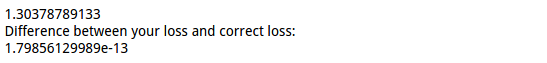
cell 4 计算包含正则的loss
1 loss, _ = net.loss(X, y, reg=0.1)
2 correct_loss = 1.30378789133
3
4 # should be very small, we get < 1e-12
5 print loss
6 print 'Difference between your loss and correct loss:'
7 print np.sum(np.abs(loss - correct_loss))
结果:
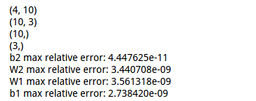
cell 5 反向传播,并用数值法来验证偏导的正确性》》注意使用链式法则:
 1 from cs231n.gradient_check import eval_numerical_gradient
 2
 3 # Use numeric gradient checking to check your implementation of the backward pass.
 4 # If your implementation is correct, the difference between the numeric and
 5 # analytic gradients should be less than 1e-8 for each of W1, W2, b1, and b2.
 6
 7 loss, grads = net.loss(X, y, reg=0.1)
 8 print  grads['W1'].shape
 9 print grads['W2'].shape
10 print grads['b1'].shape
11 print grads['b2'].shape
12 # these should all be less than 1e-8 or so
13 for param_name in grads:
14   f = lambda W: net.loss(X, y, reg=0.1)[0]
15   param_grad_num = eval_numerical_gradient(f, net.params[param_name], verbose=False)
16   print '%s max relative error: %e' % (param_name, rel_error(param_grad_num, grads[param_name]))
显示解析法与数值法的结果差异:
cell 6 训练网络模型。在loss grad 计算无误的基础上,使用对应的函数方法来训练模型。
 1 net = init_toy_model()
 2 #two layers net
 3 stats = net.train(X, y, X, y,
 4             learning_rate=1e-1, reg=1e-5,
 5             num_iters=100, verbose=False)
 6
 7 print 'Final training loss: ', stats['loss_history'][-1]
 8
 9 # plot the loss history
10 plt.plot(stats['loss_history'])
11 plt.xlabel('iteration')
12 plt.ylabel('training loss')
13 plt.title('Training Loss history')
14 plt.show()
训练函数代码:
 1   def train(self, X, y, X_val, y_val,
 2             learning_rate=1e-3, learning_rate_decay=0.95,
 3             reg=1e-5, num_iters=100,
 4             batch_size=200, verbose=False):
 5     """
 6     Train this neural network using stochastic gradient descent.
 7
 8     Inputs:
 9     - X: A numpy array of shape (N, D) giving training data.
10     - y: A numpy array f shape (N,) giving training labels; y[i] = c means that
11       X[i] has label c, where 0 <= c < C.
12     - X_val: A numpy array of shape (N_val, D) giving validation data.
13     - y_val: A numpy array of shape (N_val,) giving validation labels.
14     - learning_rate: Scalar giving learning rate for optimization.
15     - learning_rate_decay: Scalar giving factor used to decay the learning rate
16       after each epoch.
17     - reg: Scalar giving regularization strength.
18     - num_iters: Number of steps to take when optimizing.
19     - batch_size: Number of training examples to use per step.
20     - verbose: boolean; if true print progress during optimization.
21     """
22     num_train = X.shape[0]
23     iterations_per_epoch = max(num_train / batch_size, 1)
24
25     # Use SGD to optimize the parameters in self.model
26     loss_history = []
27     train_acc_history = []
28     val_acc_history = []
29
30     for it in xrange(num_iters):
31       X_batch = None
32       y_batch = None
33
34       #########################################################################
35       # TODO: Create a random minibatch of training data and labels, storing  #
36       # them in X_batch and y_batch respectively.                             #
37       #########################################################################
38       if batch_size > num_train:
39         mask = np.random.choice(num_train, batch_size, replace=True)
40       else :
41         mask = np.random.choice(num_train, batch_size, replace=False)
42       X_batch = X[mask]
43       y_batch = y[mask]
44       #########################################################################
45       #                             END OF YOUR CODE                          #
46       #########################################################################
47
48       # Compute loss and gradients using the current minibatch
49       loss, grads = self.loss(X_batch, y=y_batch, reg=reg)
50       loss_history.append(loss)
51
52       #########################################################################
53       # TODO: Use the gradients in the grads dictionary to update the         #
54       # parameters of the network (stored in the dictionary self.params)      #
55       # using stochastic gradient descent. You'll need to use the gradients   #
56       # stored in the grads dictionary defined above.                         #
57       #########################################################################
58       self.params['W1'] = self.params['W1'] - learning_rate * grads['W1']
59       self.params['b1'] = self.params['b1'] - learning_rate * grads['b1']
60       self.params['W2'] = self.params['W2'] - learning_rate * grads['W2']
61       self.params['b2'] = self.params['b2'] - learning_rate * grads['b2']
62       #########################################################################
63       #                             END OF YOUR CODE                          #
64       #########################################################################
65
66       if verbose and it % 100 == 0:
67         print 'iteration %d / %d: loss %f' % (it, num_iters, loss)
68
69       # Every epoch, check train and val accuracy and decay learning rate.
70       if it % iterations_per_epoch == 0:
71         # Check accuracy
72         train_acc = (self.predict(X_batch) == y_batch).mean()
73         val_acc = (self.predict(X_val) == y_val).mean()
74         train_acc_history.append(train_acc)
75         val_acc_history.append(val_acc)
76
77         # Decay learning rate
78         learning_rate *= learning_rate_decay
79
80     return {
81       'loss_history': loss_history,
82       'train_acc_history': train_acc_history,
83       'val_acc_history': val_acc_history,
84     }
显示最终的training loss以及绘制下降曲线:

之前都是使用比较简单的数据进行计算,接下来对cifar-10进行分类。
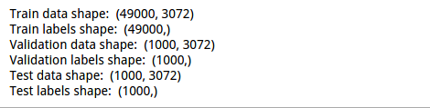
cell 7 载入训练和测试数据集,并显示各数据的维度:
 1 from cs231n.data_utils import load_CIFAR10
 2
 3 def get_CIFAR10_data(num_training=49000, num_validation=1000, num_test=1000):
 4     """
 5     Load the CIFAR-10 dataset from disk and perform preprocessing to prepare
 6     it for the two-layer neural net classifier. These are the same steps as
 7     we used for the SVM, but condensed to a single function.
 8     """
 9     # Load the raw CIFAR-10 data
10     cifar10_dir = 'cs231n/datasets/cifar-10-batches-py'
11     X_train, y_train, X_test, y_test = load_CIFAR10(cifar10_dir)
12
13     # Subsample the data
14     mask = range(num_training, num_training + num_validation)
15     X_val = X_train[mask]
16     y_val = y_train[mask]
17     mask = range(num_training)
18     X_train = X_train[mask]
19     y_train = y_train[mask]
20     mask = range(num_test)
21     X_test = X_test[mask]
22     y_test = y_test[mask]
23
24     # Normalize the data: subtract the mean image
25     mean_image = np.mean(X_train, axis=0)
26     X_train -= mean_image
27     X_val -= mean_image
28     X_test -= mean_image
29
30     # Reshape data to rows
31     X_train = X_train.reshape(num_training, -1)
32     X_val = X_val.reshape(num_validation, -1)
33     X_test = X_test.reshape(num_test, -1)
34
35     return X_train, y_train, X_val, y_val, X_test, y_test
36
37
38 # Invoke the above function to get our data.
39 X_train, y_train, X_val, y_val, X_test, y_test = get_CIFAR10_data()
40 print 'Train data shape: ', X_train.shape
41 print 'Train labels shape: ', y_train.shape
42 print 'Validation data shape: ', X_val.shape
43 print 'Validation labels shape: ', y_val.shape
44 print 'Test data shape: ', X_test.shape
45 print 'Test labels shape: ', y_test.shape
结果显示:
cell 8 初始化网络并进行训练:
 1 input_size = 32 * 32 * 3
 2 hidden_size = 50
 3 num_classes = 10
 4 net = TwoLayerNet(input_size, hidden_size, num_classes)
 5
 6 # Train the network
 7 stats = net.train(X_train, y_train, X_val, y_val,
 8             num_iters=1000, batch_size=200,
 9             learning_rate=1e-4, learning_rate_decay=0.95,
10             reg=0.5, verbose=True)
11
12 # Predict on the validation set
13 val_acc = (net.predict(X_val) == y_val).mean()
14 print 'Validation accuracy: ', val_acc
上述代码对验证集进行了预测,得到的准确率:

预测代码:
 1   def predict(self, X):
 2     """
 3     Use the trained weights of this two-layer network to predict labels for
 4     data points. For each data point we predict scores for each of the C
 5     classes, and assign each data point to the class with the highest score.
 6
 7     Inputs:
 8     - X: A numpy array of shape (N, D) giving N D-dimensional data points to
 9       classify.
10
11     Returns:
12     - y_pred: A numpy array of shape (N,) giving predicted labels for each of
13       the elements of X. For all i, y_pred[i] = c means that X[i] is predicted
14       to have class c, where 0 <= c < C.
15     """
16     W1, b1 = self.params['W1'], self.params['b1']
17     W2, b2 = self.params['W2'], self.params['b2']
18     y_pred = None
19
20     #5*10  * 10 *3 >>>5*3
21     ###########################################################################
22     # TODO: Implement this function; it should be VERY simple!                #
23     ###########################################################################
24     layer_hide = np.dot(X,W1) + b1
25     layer_hide[layer_hide<0] = 0
26     layer_soft = np.dot(layer_hide,W2) + b2
27     scores = np.subtract( layer_soft.T , np.max(layer_soft , axis = 1) ).T
28     scores = np.exp(scores)
29     scores = np.divide( scores.T , np.sum(scores , axis = 1) ).T
30     y_pred = np.argmax(scores , axis = 1)
31     ###########################################################################
32     #                              END OF YOUR CODE                           #
33     ###########################################################################
34
35     return y_pred
接下来,对网络模型进行一些调试,观察结果。
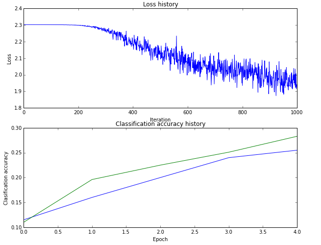
cell 9 绘制train集的loss以及train集的准确率与validation集的准确率:
 1 # Plot the loss function and train / validation accuracies
 2 plt.subplot(2, 1, 1)
 3 plt.plot(stats['loss_history'])
 4 plt.title('Loss history')
 5 plt.xlabel('Iteration')
 6 plt.ylabel('Loss')
 7
 8 plt.subplot(2, 1, 2)
 9 plt.plot(stats['train_acc_history'], label='train')
10 plt.plot(stats['val_acc_history'], label='val')
11 plt.title('Classification accuracy history')
12 plt.xlabel('Epoch')
13 plt.ylabel('Clasification accuracy')
14 plt.show()
绘制的图形曲线:
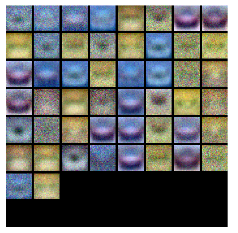
cell 10 对w的分量分别进行可视化:
 1 from cs231n.vis_utils import visualize_grid
 2
 3 # Visualize the weights of the network
 4
 5 def show_net_weights(net):
 6   W1 = net.params['W1']
 7   W1 = W1.reshape(32, 32, 3, -1).transpose(3, 0, 1, 2)
 8   plt.imshow(visualize_grid(W1, padding=3).astype('uint8'))
 9   plt.gca().axis('off')
10   plt.show()
11
12 show_net_weights(net)
结果:
接着是通过验证的方式选取超参数,包括:隐藏层的结点数、学习率、正则化强度系数。
cell 11 选取超参数,没有对正则化强度系数及其衰减系数进行选取:
 1 best_net = None # store the best model into this
 2 best_val = 0
 3 #################################################################################
 4 # TODO: Tune hyperparameters using the validation set. Store your best trained  #
 5 # model in best_net.                                                            #
 6 #                                                                               #
 7 # To help debug your network, it may help to use visualizations similar to the  #
 8 # ones we used above; these visualizations will have significant qualitative    #
 9 # differences from the ones we saw above for the poorly tuned network.          #
10 #                                                                               #
11 # Tweaking hyperparameters by hand can be fun, but you might find it useful to  #
12 # write code to sweep through possible combinations of hyperparameters          #
13 # automatically like we did on the previous exercises.                          #
14 #################################################################################
15 input_size = 32 * 32 * 3
16 Hidden_size = [50 ,64,128]
17 REG = [0.01,0.1,0.5]
18 num_classes = 10
19 for i in Hidden_size:
20     for j in REG :
21       net = TwoLayerNet(input_size,  i, num_classes)
22 # Train the network
23       stats = net.train(X_train, y_train, X_val, y_val,
24                     num_iters=2000, batch_size=200,
25                     learning_rate=1e-3, learning_rate_decay=0.95,
26                     reg = j, verbose=False)
27       val_acc = (net.predict(X_val) == y_val).mean()
28       print 'Validation accuracy: ', val_acc
29       if best_val < val_acc:
30         best_val = val_acc
31         best_net = net
32 #################################################################################
33 #                               END OF YOUR CODE                                #
34 #################################################################################
显示各个参数的验证集准确率结果:

cell 12 可视化最优参数对应模型的隐藏层结点对应的w的结果:
1 # visualize the weights of the best network
2 show_net_weights(best_net)
结果:

cell 13 使用最优参数模型对测试集进行预测:
1 test_acc = (best_net.predict(X_test) == y_test).mean()
2 print 'Test accuracy: ', test_acc
得到的结果:

附:通关CS231n企鹅群:578975100 validation:DL-CS231n