python机器学习-乳腺癌细胞挖掘(博主亲自录制视频)https://study.163.com/course/introduction.htm?courseId=1005269003&utm_campaign=commission&utm_source=cp-400000000398149&utm_medium=share

http://www.ithao123.cn/content-296918.html参考
Python 文本挖掘:简单的自然语言统计
2015-05-12 浏览(141)
[摘要:首要应用NLTK (Natural Language Toolkit)顺序包。 实在,之前正在用呆板进修方式剖析情绪的时间便已应用了简略的天然说话处置惩罚及统计。比方把分词后的文本变成单词拆配(或叫单词序]
其实,之前在用机器学习方法分析情感的时候就已经使用了简单的自然语言处理及统计。比如把分词后的文本变为双词搭配(或者叫双词序列),找出语料中出现频率最高的词,使用一定的统计方法找出信息量最丰富的词。回顾一下。
import nltk
example_1 = ['I','am','a','big','apple','.']
print nltk.bigrams(example_1)
>> [('I', 'am'), ('am', 'a'), ('a', 'big'), ('big', 'apple'), ('apple', '.')]
print nltk.trigrams(example)
>> [('I', 'am', 'a'), ('am', 'a', 'big'), ('a', 'big', 'apple'), ('big', 'apple', '.')]
from nltk.probability import FreqDist
example_2 = ['I','am','a','big','apple','.','I','am','delicious',',','I','smells','good','.','I','taste','good','.']
fdist = FreqDist(word for word in example_2) #把文本转化成词和词频的字典
print fdist.keys() #词按出现频率由高到低排列
>> ['I', '.', 'am', 'good', ',', 'a', 'apple', 'big', 'delicious', 'smells', 'taste']
print fdist.values() #语料中每个词的出现次数倒序排列
>> [4, 3, 2, 2, 1, 1, 1, 1, 1, 1, 1]
import nltk
from nltk.collocations import BigramCollocationFinder
from nltk.metrics import BigramAssocMeasures
bigrams = BigramCollocationFinder.from_words(example_2)
most_informative_chisq_bigrams = bigrams.nbest(BigramAssocMeasures.chi_sq, 3) #使用卡方统计法找
most_informative_pmi_bigrams = bigrams.nbest(BigramAssocMeasures.pmi, 3) #使用互信息方法找
print most_informative_chisq_bigrams
>> [('a', 'big'), ('big', 'apple'), ('delicious', ',')]
print most_informative_pmi_bigrams
>> [('a', 'big'), ('big', 'apple'), ('delicious', ',')]
sent_num = len(sents)
word_num = len(words)
import jieba.posseg
def postagger(sentence, para):
pos_data = jieba.posseg.cut(sentence)
pos_list = []
for w in pos_data:
pos_list.append((w.word, w.flag)) #make every word and tag as a tuple and add them to a list
return pos_list
def count_adj_adv(all_review): #只统计形容词、副词和动词的数量
adj_adv_num = []
a = 0
d = 0
v = 0
for review in all_review:
pos = tp.postagger(review, 'list')
for i in pos:
if i[1] == 'a':
a += 1
elif i[1] == 'd':
d += 1
elif i[1] == 'v':
v += 1
adj_adv_num.append((a, d, v))
a = 0
d = 0
v = 0
return adj_adv_num
from nltk.model.ngram import NgramModel
example_3 = [['I','am','a','big','apple','.'], ['I','am','delicious',','], ['I','smells','good','.','I','taste','good','.']]
train = list(itertools.chain(*example_3)) #把数据变成一个一维数组,用以训练模型
ent_per_model = NgramModel(1, train, estimator=None) #训练一元模型,该模型可计算信息熵和困惑值
def entropy_perplexity(model, dataset):
ep = []
for r in dataset:
ent = model.entropy(r)
per = model.perplexity(r)
ep.append((ent, per))
return ep
print entropy_perplexity(ent_per_model, example_3)
>> [(4.152825201361557, 17.787911185335403), (4.170127240384194, 18.002523441208137),
Entropy and Information Gain
import math,nltk
def entropy(labels):
    freqdist = nltk.FreqDist(labels)
    probs = [freqdist.freq(l) for l in freqdist]
    return -sum(p * math.log(p,2) for p in probs)
As was mentioned before, there are several methods for identifying the most informative feature for a decision stump. One popular alternative, called information gain, measures how much more organized the input values become when we divide them up using a given feature. To measure how disorganized the original set of input values are, we calculate entropy of their labels, which will be high if the input values have highly varied labels, and low if many input values all have the same label. In particular, entropy is defined as the sum of the probability of each label times the log probability of that same label:
| (1) | H = −Σl |in| labelsP(l) × log2P(l). |
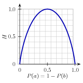
Figure 4.2: The entropy of labels in the name gender prediction task, as a function of the percentage of names in a given set that are male.
For example, 4.2 shows how the entropy of labels in the name gender prediction task depends on the ratio of male to female names. Note that if most input values have the same label (e.g., if P(male) is near 0 or near 1), then entropy is low. In particular, labels that have low frequency do not contribute much to the entropy (since P(l) is small), and labels with high frequency also do not contribute much to the entropy (since log2P(l) is small). On the other hand, if the input values have a wide variety of labels, then there are many labels with a "medium" frequency, where neither P(l) nor log2P(l) is small, so the entropy is high. 4.3 demonstrates how to calculate the entropy of a list of labels.
|
||
|
||
|
Example 4.3 (code_entropy.py): Figure 4.3: Calculating the Entropy of a List of Labels |
Once we have calculated the entropy of the original set of input values' labels, we can determine how much more organized the labels become once we apply the decision stump. To do so, we calculate the entropy for each of the decision stump's leaves, and take the average of those leaf entropy values (weighted by the number of samples in each leaf). The information gain is then equal to the original entropy minus this new, reduced entropy. The higher the information gain, the better job the decision stump does of dividing the input values into coherent groups, so we can build decision trees by selecting the decision stumps with the highest information gain.
Another consideration for decision trees is efficiency. The simple algorithm for selecting decision stumps described above must construct a candidate decision stump for every possible feature, and this process must be repeated for every node in the constructed decision tree. A number of algorithms have been developed to cut down on the training time by storing and reusing information about previously evaluated examples.
Decision trees have a number of useful qualities. To begin with, they're simple to understand, and easy to interpret. This is especially true near the top of the decision tree, where it is usually possible for the learning algorithm to find very useful features. Decision trees are especially well suited to cases where many hierarchical categorical distinctions can be made. For example, decision trees can be very effective at capturing phylogeny trees.
However, decision trees also have a few disadvantages. One problem is that, since each branch in the decision tree splits the training data, the amount of training data available to train nodes lower in the tree can become quite small. As a result, these lower decision nodes may
overfit the training set, learning patterns that reflect idiosyncrasies of the training set rather than linguistically significant patterns in the underlying problem. One solution to this problem is to stop dividing nodes once the amount of training data becomes too small. Another solution is to grow a full decision tree, but then to prune decision nodes that do not improve performance on a dev-test.
A second problem with decision trees is that they force features to be checked in a specific order, even when features may act relatively independently of one another. For example, when classifying documents into topics (such as sports, automotive, or murder mystery), features such as hasword(football) are highly indicative of a specific label, regardless of what other the feature values are. Since there is limited space near the top of the decision tree, most of these features will need to be repeated on many different branches in the tree. And since the number of branches increases exponentially as we go down the tree, the amount of repetition can be very large.
A related problem is that decision trees are not good at making use of features that are weak predictors of the correct label. Since these features make relatively small incremental improvements, they tend to occur very low in the decision tree. But by the time the decision tree learner has descended far enough to use these features, there is not enough training data left to reliably determine what effect they should have. If we could instead look at the effect of these features across the entire training set, then we might be able to make some conclusions about how they should affect the choice of label.
The fact that decision trees require that features be checked in a specific order limits their ability to exploit features that are relatively independent of one another. The naive Bayes classification method, which we'll discuss next, overcomes this limitation by allowing all features to act "in parallel."
https://study.163.com/provider/400000000398149/index.htm?share=2&shareId=400000000398149(博主视频教学主页)