Python/spss-多元回归建模-共线性诊断2（推荐AA）

 

python风控建模实战lendingClub(博主录制，包含大量回归建模脚本，2K超清分辨率)

https://study.163.com/course/courseMain.htm?courseId=1005988013&share=2&shareId=400000000398149

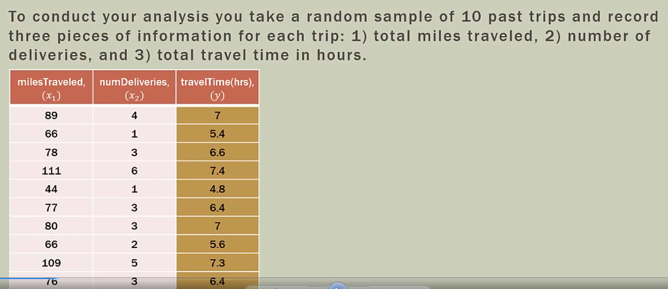
多元共线性

在一个回归方程中，假如两个或两个以上解释变量彼此高度相关，那么回归分析的结果将有可能无法分清每一个变量与因变量之间的真实关系。例如我们要知道吸毒对SAT考试分数的影响，我们会询问对象是否吸收过可卡因或海洛因，并用软件计算它们之间的系数。

虽然求出了海洛因和可卡因额回归系数，但两者相关性发生重叠，使R平方变大，依然无法揭开真实的情况。
因为吸食海洛因的人常常吸食可卡因，单独吸食一种毒品人很少。

当两个变量高度相关时，我们通常在回归方程中只采用其中一个，或创造一个新的综合变量，如吸食可卡因或海洛因。

又例如当研究员想要控制学生的整体经济背景时，他们会将父母双方的受教育程度都纳入方程式中。

如果单独把父亲或母亲的教育程度分离考虑，会引起混淆，分析变得模糊，因为丈夫和妻子的教育程度有很大相关性。

 
多元共线性带来问题：
（1）自变量不显著
（2）参数估计值的正负号产生影响
 

共线性统计量：
（1）容忍度tolerance
         tolerance<0.1 表示存在严重多重共线
（2）方差扩大因子 variance inflation factor （VIF）
         VIF>10表示存在严重多重共线性

 自变量为x1和x2时

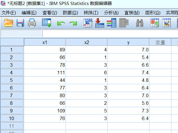
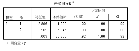
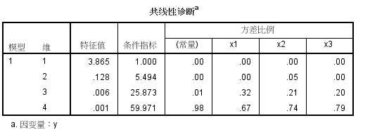
spss共线性诊断

spss导入excel数据

条件指数第三个为30.866，大于10，说明共线性很高

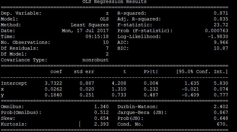
F检验是对整个模型而已的，看是不是自变量系数不全为0，这里F检验值23，对应P概率=0，P<0.05,H1成立，说明显著性非常高

t检验则是分别针对某个自变量的，看每个自变量是否有显著预测效力。这里t检验对应概率大于0.05，为0.23和0.48，说明显著性很差

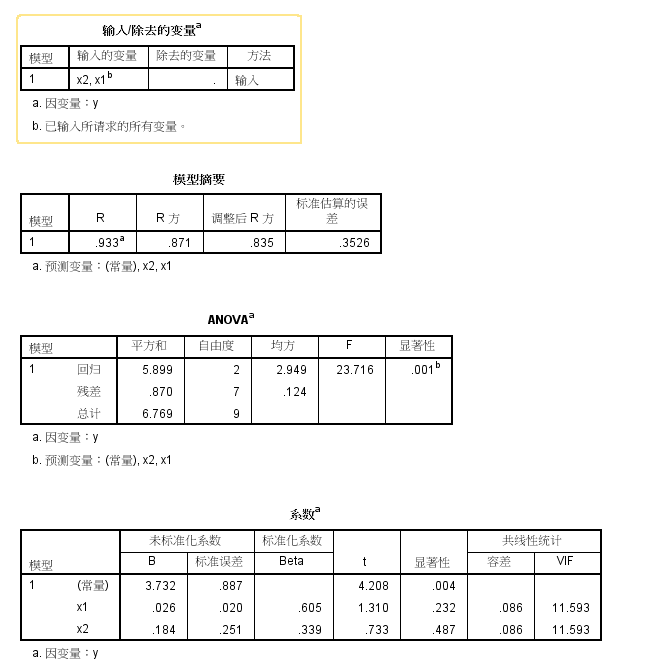
 x1 的t分数p值0.232，P值>0.05,不否定H0假设，显著性不高

  x2 的t分数p值0.487，P值>0.05,不否定H0假设，显著性不高

Python脚本分析

condition num=670 ，未能检测出共线性

Python目前支持2D和3D绘图，可解决两元回归绘图。但目前没发现4D绘图，即解决三元回归及其以上绘图

# -*- coding: utf-8 -*-
"""
Created on Fri Feb 23 16:54:54 2018

@author: Administrator
"""

# Import standard packages
import numpy as np
import matplotlib.pyplot as plt
import pandas as pd
import seaborn as sns
from sklearn import datasets, linear_model
from matplotlib.font_manager import FontProperties 
font_set = FontProperties(fname=r"c:windowsfontssimsun.ttc", size=15)  
# additional packages
import sys
import os
sys.path.append(os.path.join('..', '..', 'Utilities'))

try:
# Import formatting commands if directory "Utilities" is available
    from ISP_mystyle import showData 
    
except ImportError:
# Ensure correct performance otherwise
    def showData(*options):
        plt.show()
        return

# additional packages ...
# ... for the 3d plot ...
from mpl_toolkits.mplot3d import Axes3D
from matplotlib import cm

# ... and for the statistic
from statsmodels.formula.api import ols
#生成组合
from itertools import combinations

x1=[5,2,4,2.5,3,3.5,2.5,3]
x2=[1.5,2,1.5,2.5,3.3,2.3,4.2,2.5]
y=[96,90,95,92,95,94,94,94]


#自变量列表
list_x=[x1,x2]

#绘制多元回归三维图
def Draw_multilinear():
    
    df = pd.DataFrame({'x1':x1,'x2':x2,'y':y})
    # --- >>> START stats <<< ---
    # Fit the model
    model = ols("y~x1+x2", df).fit()
    param_intercept=model.params[0]
    param_x1=model.params[1]
    param_x2=model.params[2]
    rSquared_adj=model.rsquared_adj
    
    #generate data,产生矩阵然后把数值附上去
    x = np.linspace(-5,5,101)
    (X,Y) = np.meshgrid(x,x)
    
    # To get reproducable values, I provide a seed value
    np.random.seed(987654321)   
    Z = param_intercept + param_x1*X+param_x2*Y+np.random.randn(np.shape(X)[0], np.shape(X)[1])

    # 绘图
    #Set the color
    myCmap = cm.GnBu_r
    # If you want a colormap from seaborn use:
    #from matplotlib.colors import ListedColormap
    #myCmap = ListedColormap(sns.color_palette("Blues", 20))
    
    # Plot the figure
    fig = plt.figure("multi")
    ax = fig.gca(projection='3d')
    surf = ax.plot_surface(X,Y,Z, cmap=myCmap, rstride=2, cstride=2, 
        linewidth=0, antialiased=False)
    ax.view_init(20,-120)
    ax.set_xlabel('X')
    ax.set_ylabel('Y')
    ax.set_zlabel('Z')
    ax.set_title("multilinear with adj_Rsquare %f"%(rSquared_adj))
    fig.colorbar(surf, shrink=0.6)
    
    outFile = '3dSurface.png'
    showData(outFile)

    
#检查独立变量之间共线性关系
def Two_dependentVariables_compare(x1,x2):
    # Convert the data into a Pandas DataFrame
    df = pd.DataFrame({'x':x1, 'y':x2})
    # Fit the model
    model = ols("y~x", df).fit()
    rSquared_adj=model.rsquared_adj
    print("rSquared_adj",rSquared_adj)
    if rSquared_adj>=0.8:
        print("high relation")
        return True
    elif 0.6<=rSquared_adj<0.8:
         print("middle relation")
         return False
    elif rSquared_adj<0.6:
         print("low relation")
         return False

#比较所有参数，观察是否存在多重共线
def All_dependentVariables_compare(list_x):  
    list_status=[]
    list_combine=list(combinations(list_x, 2))
    for i in list_combine:
        x1=i[0]
        x2=i[1]
        status=Two_dependentVariables_compare(x1,x2)
        list_status.append(status)
    if True in list_status:
        print("there is multicorrelation exist in dependent variables")
        return True
    else:
        return False
    
        
#回归方程，支持哑铃变量
def regressionModel(x1,x2,y):
    '''Multilinear regression model, calculating fit, P-values, confidence intervals etc.'''
    # Convert the data into a Pandas DataFrame
    df = pd.DataFrame({'x1':x1,'x2':x2,'y':y})
    
    # --- >>> START stats <<< ---
    # Fit the model
    model = ols("y~x1+x2", df).fit()
    # Print the summary
    print((model.summary()))
    return model._results.params  # should be array([-4.99754526,  3.00250049, -0.50514907])

    
# Function to show the resutls of linear fit model
def Draw_linear_line(X_parameters,Y_parameters,figname,x1Name,x2Name):
    #figname表示图表名字，用于生成独立图表fig1 = plt.figure('fig1')，fig2 = plt.figure('fig2')
    plt.figure(figname)
    #获取调整R方参数    
    df = pd.DataFrame({'x':X_parameters, 'y':Y_parameters})
    # Fit the model
    model = ols("y~x", df).fit()
    rSquared_adj=model.rsquared_adj 
    
    #处理X_parameter1数据
    X_parameter1 = []
    for i in X_parameters:
        X_parameter1.append([i])
    
    # Create linear regression object
    regr = linear_model.LinearRegression()
    regr.fit(X_parameter1, Y_parameters)
    plt.scatter(X_parameter1,Y_parameters,color='blue',label="real value")
    plt.plot(X_parameter1,regr.predict(X_parameter1),color='red',linewidth=4,label="prediction line")
    plt.title("linear regression %s and %s with adj_rSquare:%f"%(x1Name,x2Name,rSquared_adj))
    plt.xlabel('x', fontproperties=font_set)  
    plt.ylabel('y', fontproperties=font_set)  
    plt.xticks(())
    plt.yticks(())
    plt.legend()
    plt.show()      
    

#绘制多元回归三维图
Draw_multilinear()  
#比较所有参数，观察是否存在多重共线
All_dependentVariables_compare(list_x)              
Draw_linear_line(x1,x2,"fig1","x1","x2")
Draw_linear_line(x1,y,"fig4","x1","y")
Draw_linear_line(x2,y,"fig5","x2","y")
regressionModel(x1,x2,y)

　　

当自变量为x1,x2,x3三个时

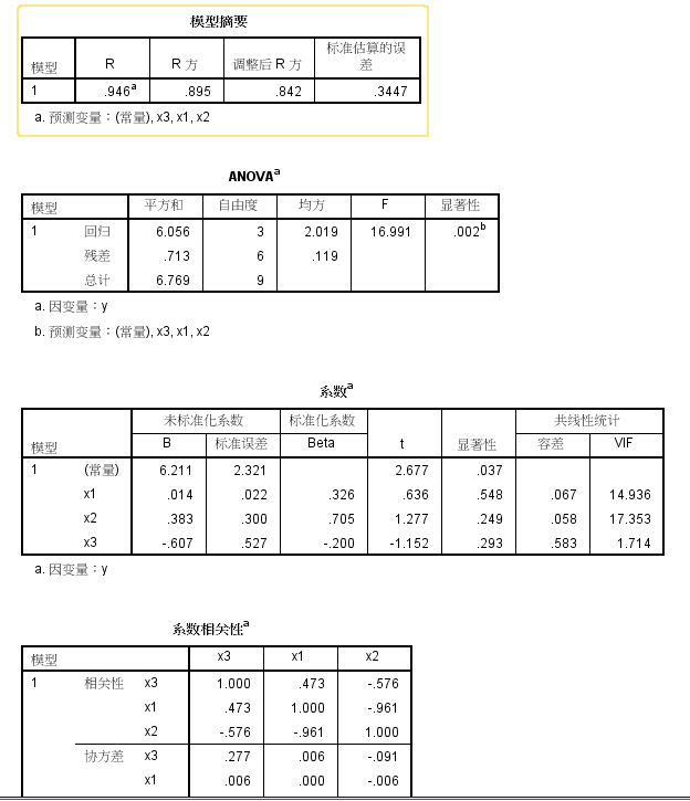
spss分析

python脚本

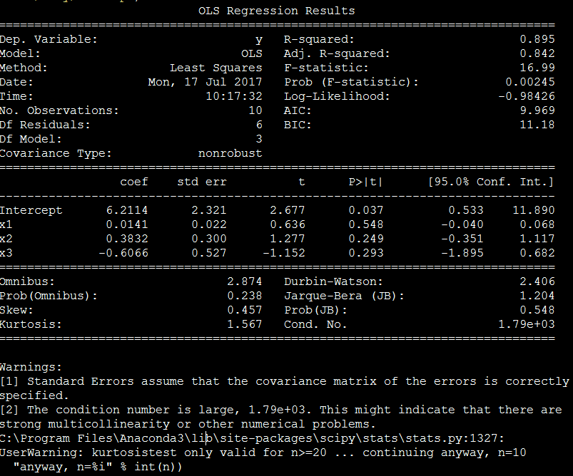
程序运行后，cond.no数值过高，提醒有多重共线可能

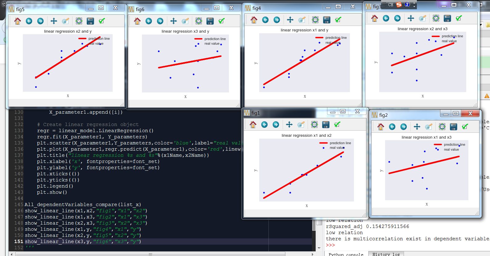
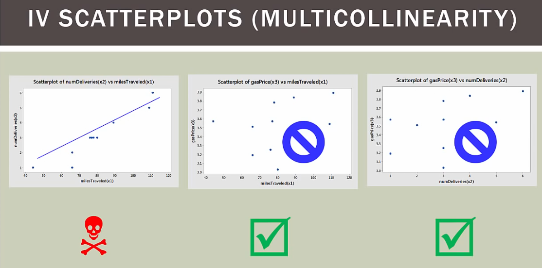
可视化分析

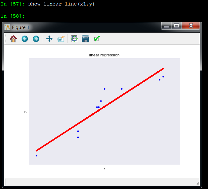
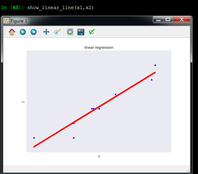
x1和y成线性关系

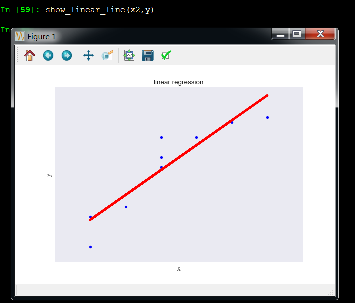
x2和y成线性关系

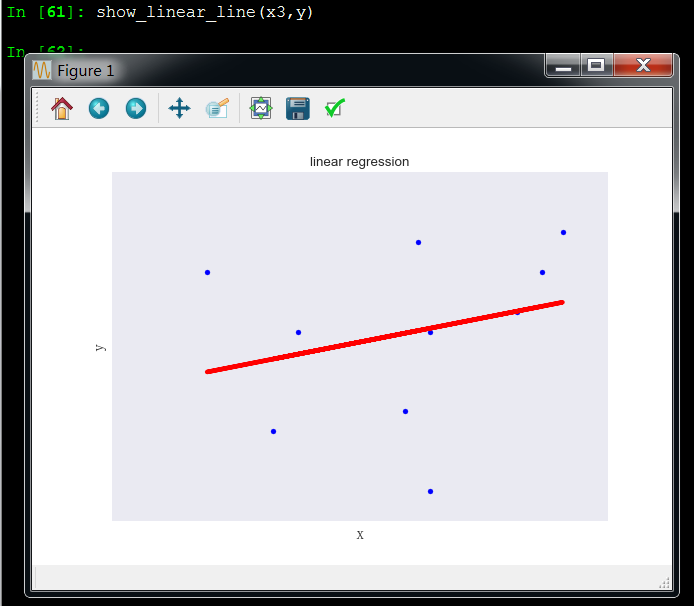
x3和y成非线性关系，所以x3变量应该剔除，和y没啥关系

x1和x2成线性关系,这引起了多重共线性问题

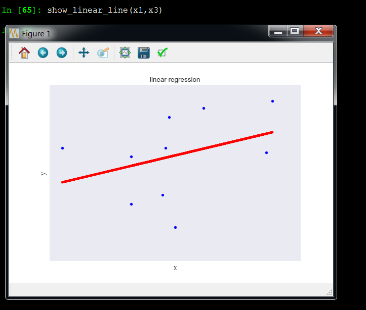
x1和x3成非线性关系

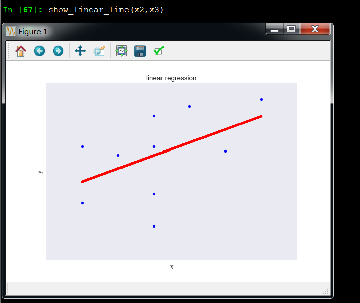
x2和x3成非线性关系

 

multiLinearIsBetterThanSimpleLinearRegression1.py

从excel调取数据，适用于数据量百万级分析

# -*- coding: utf-8 -*-
"""
Created on Fri Feb 23 16:54:54 2018

@author: Toby QQ:231469242
多元回归的多重共线性检测，数据可视化
"""

# Import standard packages
import matplotlib.pyplot as plt
import pandas as pd
from sklearn import linear_model
from matplotlib.font_manager import FontProperties 
font_set = FontProperties(fname=r"c:windowsfontssimsun.ttc", size=15)  
# ... and for the statistic
from statsmodels.formula.api import ols
#生成组合
from itertools import combinations


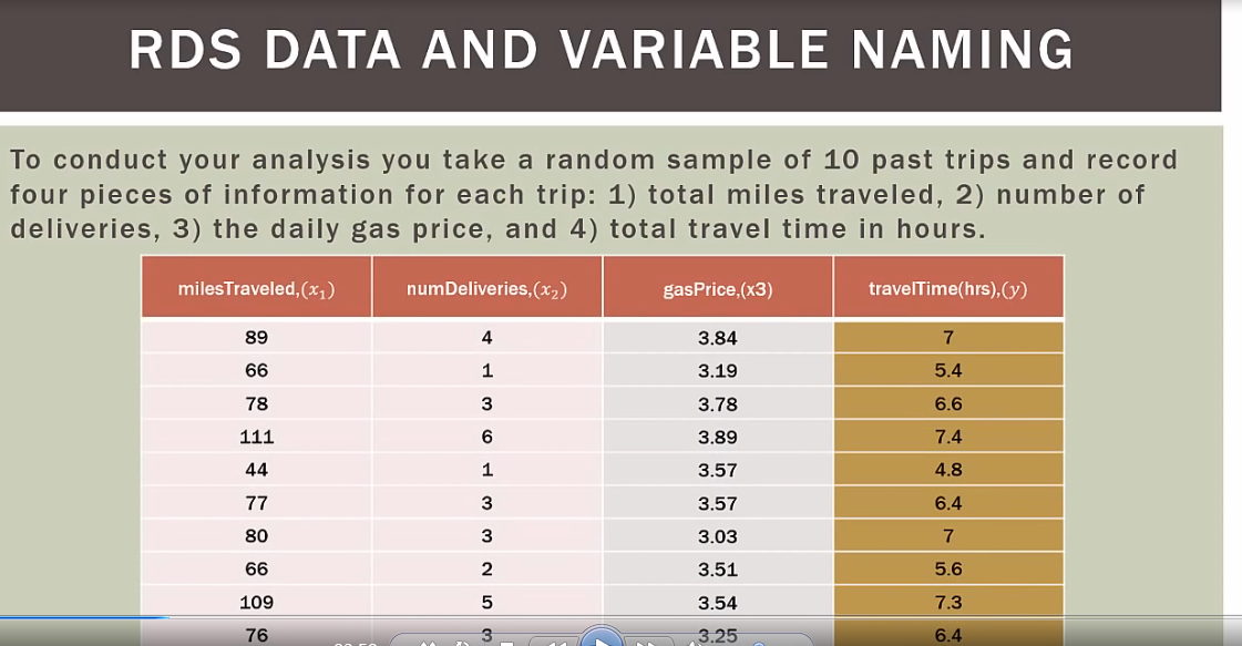
df=pd.read_excel("旅行公里-投递数量-行驶时间.xlsx")  
array_values=df.values
x1=[i[0] for i in array_values]
x2=[i[1] for i in array_values]
x3=[i[2] for i in array_values]
y=[i[3] for i in array_values]
sample=len(x1)
#自变量列表
list_x=[x1,x2]


#检查独立变量之间共线性关系，如果两个变量有共线性返回TRUE，反之返回FALSE
def Two_dependentVariables_compare(x1,x2):
    # Convert the data into a Pandas DataFrame
    df = pd.DataFrame({'x':x1, 'y':x2})
    # Fit the model
    model = ols("y~x", df).fit()
    rSquared_adj=model.rsquared_adj
    print("rSquared_adj",rSquared_adj)
    if rSquared_adj>=0.8:
        print("high relation")
        return True
    elif 0.6<=rSquared_adj<0.8:
         print("middle relation")
         return False
    elif rSquared_adj<0.6:
         print("low relation")
         return False

#比较所有参数，观察是否存在多重共线
def All_dependentVariables_compare(list_x):  
    list_status=[]
    #对变量列表的多个自变量进行组合，2个为一组
    list_combine=list(combinations(list_x, 2))
    for i in list_combine:
        x1=i[0]
        x2=i[1]
        status=Two_dependentVariables_compare(x1,x2)
        list_status.append(status)
    if True in list_status:
        print("there is multicorrelation exist in dependent variables")
        return True
    else:
        return False
    
        
#回归方程，支持哑铃变量,这个函数是有三个自变量，自变量个数可以自己改
def regressionModel(x1,x2,x3,y):
    '''Multilinear regression model, calculating fit, P-values, confidence intervals etc.'''
     
    # Convert the data into a Pandas DataFrame
    df = pd.DataFrame({'x1':x1, 'x2':x2,'x3':x3,'y':y})
     
    # --- >>> START stats <<< ---
    # Fit the model
    model = ols("y~x1+x2+x3", df).fit()
    # Print the summary
    print((model.summary()))
    # --- >>> STOP stats <<< ---
    return model._results.params  # should be array([-4.99754526,  3.00250049, -0.50514907])

    
# Function to show the resutls of linear fit model
def Draw_linear_line(X_parameters,Y_parameters,figname,x1Name,x2Name):
    #figname表示图表名字，用于生成独立图表fig1 = plt.figure('fig1')，fig2 = plt.figure('fig2')
    plt.figure(figname)
    #获取调整R方参数    
    df = pd.DataFrame({'x':X_parameters, 'y':Y_parameters})
    # Fit the model
    model = ols("y~x", df).fit()
    rSquared_adj=model.rsquared_adj 
    
    #处理X_parameter1数据
    X_parameter1 = []
    for i in X_parameters:
        X_parameter1.append([i])
    
    # Create linear regression object
    regr = linear_model.LinearRegression()
    regr.fit(X_parameter1, Y_parameters)
    plt.scatter(X_parameter1,Y_parameters,color='blue',label="real value")
    plt.plot(X_parameter1,regr.predict(X_parameter1),color='red',linewidth=4,label="prediction line")
    plt.title("linear regression %s and %s with adj_rSquare:%f"%(x1Name,x2Name,rSquared_adj))
    plt.xlabel('x', fontproperties=font_set)  
    plt.ylabel('y', fontproperties=font_set)  
    plt.xticks(())
    plt.yticks(())
    plt.legend()
    plt.show()      
    


#比较所有参数，观察是否存在多重共线
All_dependentVariables_compare(list_x)  
#两个变量散点图可视化            
Draw_linear_line(x1,x2,"fig1","x1","x2")
Draw_linear_line(x1,x3,"fig2","x1","x3")
Draw_linear_line(x2,x3,"fig3","x2","x3")
Draw_linear_line(x1,y,"fig4","x1","y")
Draw_linear_line(x2,y,"fig5","x2","y")
Draw_linear_line(x3,y,"fig6","x3","y")
#回归分析
regressionModel(x1,x2,x3,y)

多元回归共线性详细解释

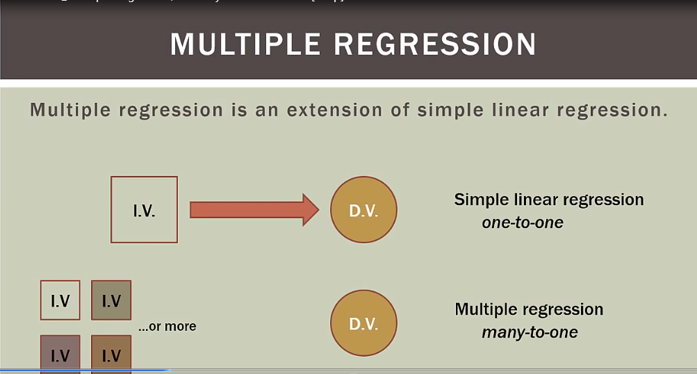
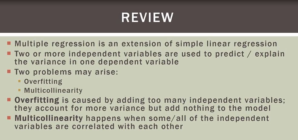
多元回归是一元回归升级版，含有多个变量

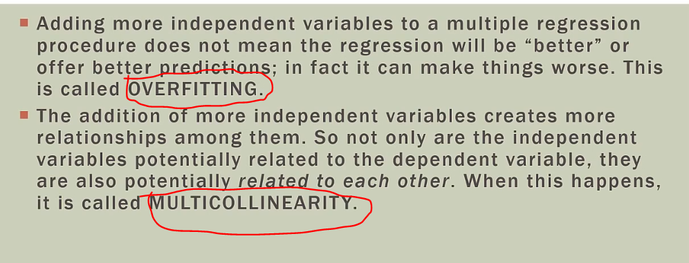
overffiting:过多独立变量不一定会让模型更好，事实上可能更糟

multicollinearity:变量之间互相关联，造成多重共线

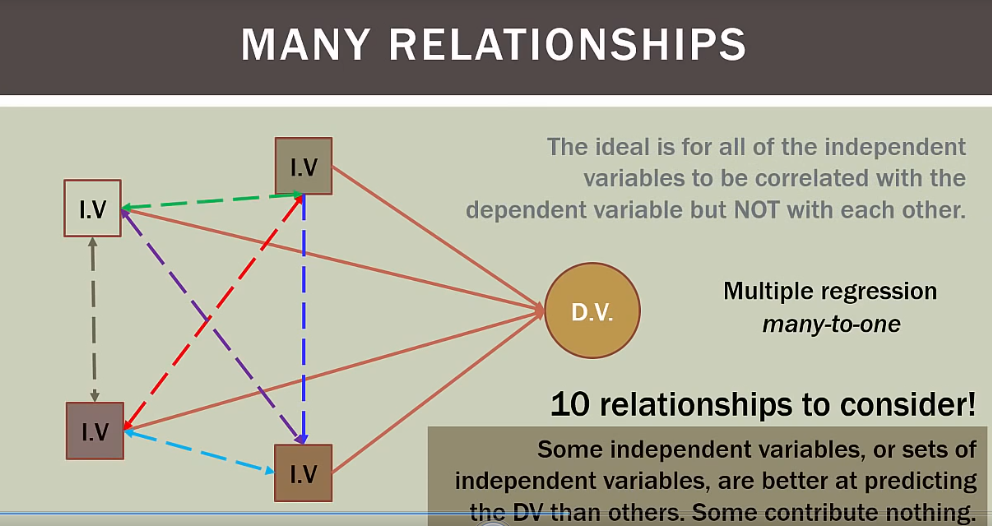
理想模型是所有独立变量和依赖变量都相关，但独立变量之间不能相互关联，独立变量必须独立

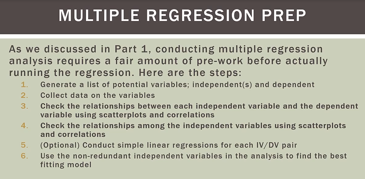
多元回归有很多事前工作做，包括发行overffitng和multilinear

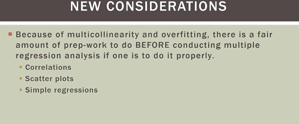
独立变量之间有潜在的多重共线可能

如果有四个变量，就有十种关系考虑

总结

 

 

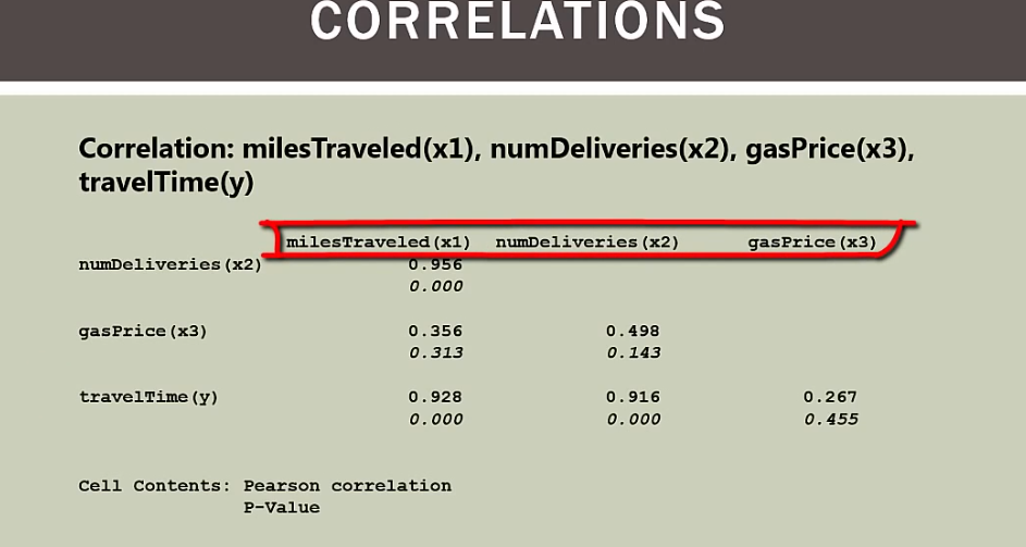
x1和x2有多重共线性

python信用评分卡建模（附代码，博主录制）

https://study.163.com/course/introduction.htm?courseId=1005214003&utm_campaign=commission&utm_source=cp-400000000398149&utm_medium=share

微信扫二维码，免费学习更多python资源