神经网络2-预测药物靶点

 python机器学习-乳腺癌细胞挖掘（博主亲自录制视频）

https://study.163.com/course/introduction.htm?courseId=1005269003&utm_campaign=commission&utm_source=cp-400000000398149&utm_medium=share

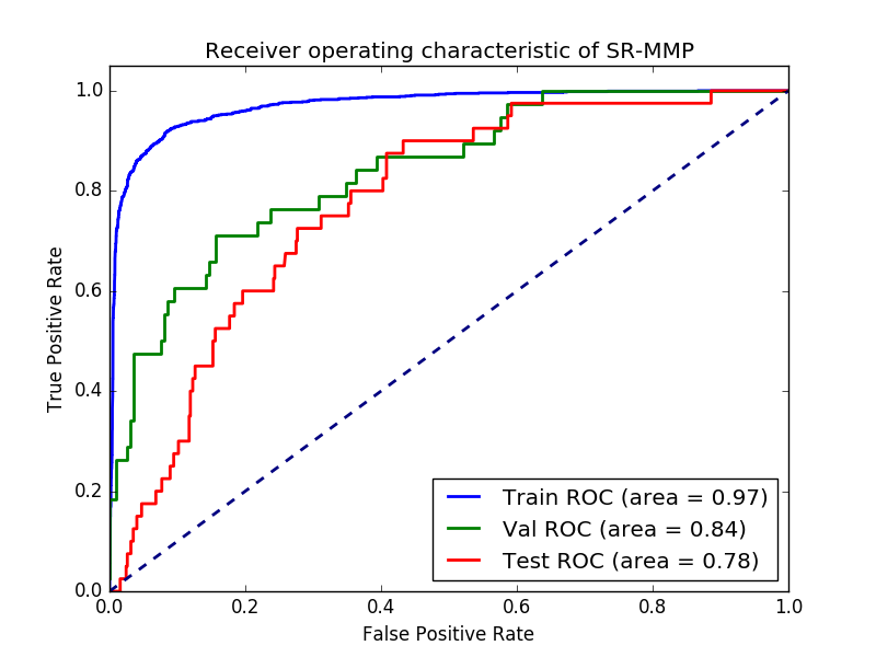
结论：神经网络算法有过度拟合，尝试其他算法，x_test和y_test报错

# -*- coding: utf-8 -*-
"""
Created on Wed Sep  5 11:23:58 2018

@author: zhi.li04
数据源与说明文档
https://www.wildcardconsulting.dk/useful-information/a-deep-tox21-neural-network-with-rdkit-and-keras/
"""
import pandas as pd
import numpy as np
 
#RDkit for fingerprinting and cheminformatics
from rdkit import Chem, DataStructs
from rdkit.Chem import AllChem, rdMolDescriptors
 
#MolVS for standardization and normalization of molecules
import molvs as mv



#Function to get parent of a smiles
def parent(smiles):
 st = mv.Standardizer() #MolVS standardizer
 try:
  mols = st.charge_parent(Chem.MolFromSmiles(smiles))
  return Chem.MolToSmiles(mols)
 except:
  print "%s failed conversion"%smiles
  return "NaN"
 
#Clean and standardize the data
def clean_data(data):
 #remove missing smiles
 data = data[~(data['smiles'].isnull())]
 
 #Standardize and get parent with molvs
 data["smiles_parent"] = data.smiles.apply(parent)
 data = data[~(data['smiles_parent'] == "NaN")]
 
 #Filter small fragents away
 def NumAtoms(smile):
  return Chem.MolFromSmiles(smile).GetNumAtoms()
 
 data["NumAtoms"] = data["smiles_parent"].apply(NumAtoms)
 data = data[data["NumAtoms"] > 3]
 return data
 


#Read the data
data = pd.DataFrame.from_csv('tox21_10k_data_all_pandas.csv')
valdata = pd.DataFrame.from_csv('tox21_10k_challenge_test_pandas.csv')
testdata = pd.DataFrame.from_csv('tox21_10k_challenge_score_pandas.csv')

data = clean_data(data)
valdata = clean_data(valdata)
testdata = clean_data(testdata)


#Calculate Fingerprints
def morgan_fp(smiles):
 mol = Chem.MolFromSmiles(smiles)
 fp = AllChem.GetMorganFingerprintAsBitVect(mol,3, nBits=8192)
 npfp = np.array(list(fp.ToBitString())).astype('int8')
 return npfp
 
fp = "morgan"
data[fp] = data["smiles_parent"].apply(morgan_fp) 
valdata[fp] = valdata["smiles_parent"].apply(morgan_fp) 
testdata[fp] = testdata["smiles_parent"].apply(morgan_fp) 


#Choose property to model
prop = 'SR-MMP'
 
#Convert to Numpy arrays
X_train = np.array(list(data[~(data[prop].isnull())][fp]))
X_val = np.array(list(valdata[~(valdata[prop].isnull())][fp]))
X_test = np.array(list(testdata[~(testdata[prop].isnull())][fp]))
 
#Select the property values from data where the value of the property is not null and reshape
y_train = data[~(data[prop].isnull())][prop].values.reshape(-1,1)
y_val = valdata[~(valdata[prop].isnull())][prop].values.reshape(-1,1)
y_test = testdata[~(testdata[prop].isnull())][prop].values.reshape(-1,1)

#Set network hyper parameters
l1 = 0.000
l2 = 0.016
dropout = 0.5
hidden_dim = 80
 
#Build neural network
model = Sequential()
model.add(Dropout(0.2, input_shape=(X_train.shape[1],)))
for i in range(3):
 wr = WeightRegularizer(l2 = l2, l1 = l1) 
 model.add(Dense(output_dim=hidden_dim, activation="relu", W_regularizer=wr))
 model.add(Dropout(dropout))
wr = WeightRegularizer(l2 = l2, l1 = l1) 
model.add(Dense(y_train.shape[1], activation='sigmoid',W_regularizer=wr))
 
##Compile model and make it ready for optimization
model.compile(loss='binary_crossentropy', optimizer = SGD(lr=0.005, momentum=0.9, nesterov=True), metrics=['binary_crossentropy'])
#Reduce lr callback
reduce_lr = ReduceLROnPlateau(monitor='loss', factor=0.5,patience=50, min_lr=0.00001, verbose=1)
 
#Training
history = model.fit(X_train, y_train, nb_epoch=1000, batch_size=1000, validation_data=(X_val,y_val), callbacks=[reduce_lr])



#Plot Train History
def plot_history(history):
    lw = 2
    fig, ax1 = plt.subplots()
    ax1.plot(history.epoch, history.history['binary_crossentropy'],c='b', label="Train", lw=lw)
    ax1.plot(history.epoch, history.history['val_loss'],c='g', label="Val", lw=lw)
    plt.ylim([0.0, max(history.history['binary_crossentropy'])])
    ax1.set_xlabel('Epochs')
    ax1.set_ylabel('Loss')
    ax2 = ax1.twinx()
    ax2.plot(history.epoch, history.history['lr'],c='r', label="Learning Rate", lw=lw)
    ax2.set_ylabel('Learning rate')
    plt.legend()
    plt.show()
 
plot_history(history)


def show_auc(model):
    pred_train = model.predict(X_train)
    pred_val = model.predict(X_val)
    pred_test = model.predict(X_test)
 
    auc_train = roc_auc_score(y_train, pred_train)
    auc_val = roc_auc_score(y_val, pred_val)
    auc_test = roc_auc_score(y_test, pred_test)
    print "AUC, Train:%0.3F Test:%0.3F Val:%0.3F"%(auc_train, auc_test, auc_val)
 
    fpr_train, tpr_train, _ =roc_curve(y_train, pred_train)
    fpr_val, tpr_val, _ = roc_curve(y_val, pred_val)
    fpr_test, tpr_test, _ = roc_curve(y_test, pred_test)
 
    plt.figure()
    lw = 2
    plt.plot(fpr_train, tpr_train, color='b',lw=lw, label='Train ROC (area = %0.2f)'%auc_train)
    plt.plot(fpr_val, tpr_val, color='g',lw=lw, label='Val ROC (area = %0.2f)'%auc_val)
    plt.plot(fpr_test, tpr_test, color='r',lw=lw, label='Test ROC (area = %0.2f)'%auc_test)
 
    plt.plot([0, 1], [0, 1], color='navy', lw=lw, linestyle='--')
    plt.xlim([0.0, 1.0])
    plt.ylim([0.0, 1.05])
    plt.xlabel('False Positive Rate')
    plt.ylabel('True Positive Rate')
    plt.title('Receiver operating characteristic of %s'%prop)
    plt.legend(loc="lower right")
    plt.interactive(True)
    plt.show()
 
show_auc(model)


#Compare with a Linear model
from sklearn import linear_model
#prepare scoring lists
fitscores = []
predictscores = []
##prepare a log spaced list of alpha values to test
alphas = np.logspace(-2, 4, num=10)
##Iterate through alphas and fit with Ridge Regression
for alpha in alphas:
  estimator = linear_model.LogisticRegression(C = 1/alpha)
  estimator.fit(X_train,y_train)
  fitscores.append(estimator.score(X_train,y_train))
  predictscores.append(estimator.score(X_val,y_val))
 
#show a plot
import matplotlib.pyplot as plt
ax = plt.gca()
ax.set_xscale('log')
ax.plot(alphas, fitscores,'g')
ax.plot(alphas, predictscores,'b')
plt.xlabel('alpha')
plt.ylabel('Correlation Coefficient')
plt.show()
 
estimator= linear_model.LogisticRegression(C = 1)
estimator.fit(X_train,y_train)
#Predict the test set
y_pred = estimator.predict(X_test)
print roc_auc_score(y_test, y_pred)

　　

 https://study.163.com/provider/400000000398149/index.htm?share=2&shareId=400000000398149（ 欢迎关注博主主页，学习python视频资源，还有大量免费python经典文章）

 

机器学习项目合作QQ:231469242