摘要
对于DNN,大多数时间我们都只需要利用成熟的第三方库配置网络结构和超参就能实现我们想要的模型。
底层的求导、梯度下降永远是一个黑盒,我们不知道发生了什么,只知道使用optimizer使loss函数收敛,得到好的模型表现能力。
本文从零开始,实现DNN网络中需要的各种操作,拼凑出一个简单的模型在iris数据集上验证效果。
梯度
什么是梯度
梯度是一个向量,指向函数值下降最快的方向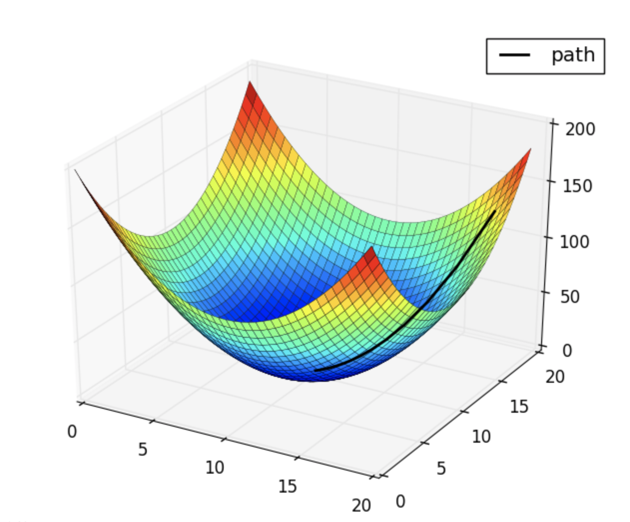
如果将函数图像视为一个实体面,梯度近似于水自由流动的方向,向着这个方向走能最快得到最的小函数值。
从数值上来讲,梯度的每一个分量分别对应该点在该轴方向上的偏导数

偏导数链式求导法则
想象一下这样一个公式
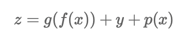
对x求导得

x的偏导数等于包含x项的导数之和
复合函数求导等于外层函数导数与内层函数导数之积 这个法则称为链式求导法则
矩阵求导法则
矩阵乘法实际上是多项式乘法的另一种直观写法
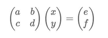
其实是由两个多项式函数组成
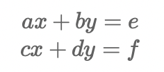
对x,y进行求偏导写成矩阵的形式为
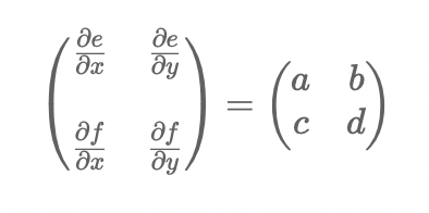
该矩阵被称为jacobian矩阵
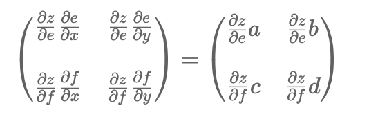
若e,f会被带到外层函数中继续参与计算 得到最终结果z
根据链式求导法则,z对xy求导的jacobian矩阵为
最终x,y的偏导数为
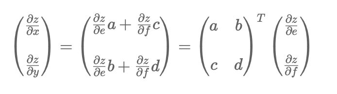
假设矩阵(e f)的导数为G 输入矩阵(a b, c d)为I 则x y的梯度应该为
![]()
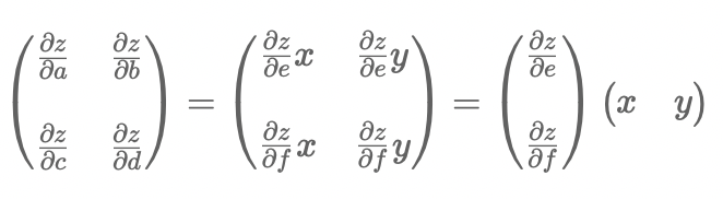
若a,b,c,d不是常数而是复合函数 则a,b,c,d也有对应的偏导数 其jacobian矩阵为
实现
基本操作实现
使用了numpy库用作矩阵操作,pandas库用来读取iris数据集,没有使用现有机器学习库
import numpy as np
import pandas as pd

# 定义各种操作的基类
class Operation:
    def __init__(self):
        self.inp = np.zeros(0)

    # 前向生成结果 inp为输入 返回值为操作的计算结果
    def forward(self, inp):
        self.inp = inp

    # 反向求导生成梯度 grad为出参的导数矩阵(链式求导法则的系数) 返回值为入参的导数矩阵
    def backward(self, grad):
        pass

    # 模仿pytorch形式的调用方式
    def __call__(self, *args, **kwargs):
        return self.forward(args[0])
class Linear(Operation):

    def __init__(self, inp_size, out_size):
        super().__init__()
        self.k = np.random.rand(inp_size, out_size) - 0.5
        self.k_grad = np.zeros((inp_size, out_size)) - 0.5
        self.b = np.random.rand(out_size) - 0.5
        self.b_grad = np.zeros(out_size) - 0.5

    def forward(self, inp):
        super().forward(inp)
        return np.matmul(inp, self.k) + self.b

    def backward(self, grad):
        self.b_grad = grad.sum(axis=0) # b的jacobian矩阵
        self.k_grad = np.matmul(self.inp.transpose(), grad) # k的jacobian矩阵
        return np.matmul(grad, self.k.transpose()) # 入参的jacobian矩阵
线性函数y=kx+b
由于操作包含两个变量矩阵k,b 在backward方法中不仅要对入参进行求导 也需要对这两个参数进行求导 求导法则参照上文矩阵求导法则部分
class ReLU(Operation):

    def __init__(self):
        super().__init__()

    def forward(self, inp):
        super().forward(inp)
        inp[inp < 0] = 0
        return inp

    def backward(self, grad):
        grad[self.inp < 0] = 0
        return grad
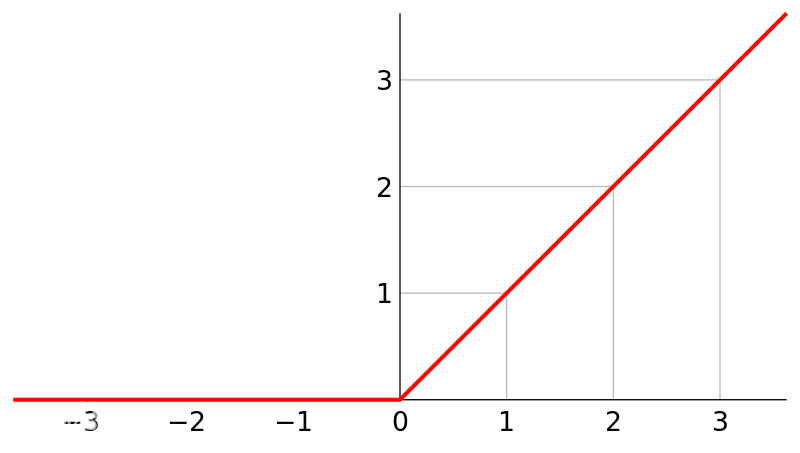
非线性函数ReLU本身是一个max(0, x)前向操作将负数置为0即可
反向求梯度操作,饱和部分梯度为0 非饱和部分梯度为1 将输入中负数部分对应的出参导数置为0即为入参导数矩阵
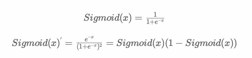
class Sigmoid(Operation):

    def __init__(self):
        super().__init__()

    def forward(self, inp):
        super().forward(inp)
        return 1 / (np.exp(-inp) + 1)

    def backward(self, grad):
        output = 1 / (np.exp(-self.inp) + 1)
        return out(1-out) * grad
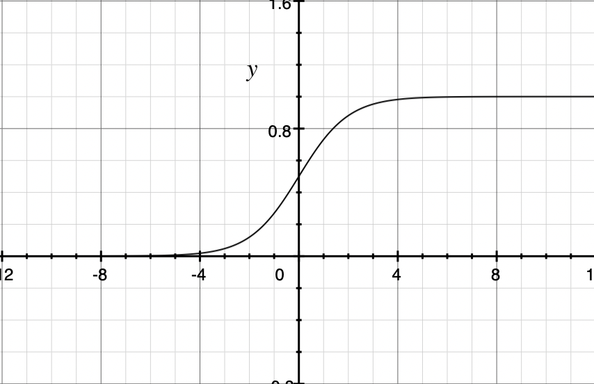
Sigmoid函数,这里使用其主要目的是生成概率。
Sigmoid可以将函数值映射到0-1之间,可以将网络计算的数值结果映射成概率结果 其导数为
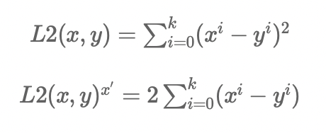
class L2Loss(Operation):

    def __init__(self, label):
        super().__init__()
        self.label = label

    def forward(self, inp):
        super().forward(inp)
        return np.power((inp - self.label), 2).sum()

    def backward(self, grad):
        return 2 * (self.inp - self.label) * grad
L2 loss 用来定义损失函数
DNN模型实现
class Dnn:

    # 模型定义 input->hidden_layer[ReLU]->output[Sigmoid]
    def __init__(self, inp_size, hidden_nodes, batch_size):
        self.l1 = Linear(inp_size, hidden_nodes)
        self.relu = ReLU()
        self.l2 = Linear(hidden_nodes, 1)
        self.sigmoid = Sigmoid()
        self.loss = L2Loss([])
        self.batch_size = batch_size

    # 计算模型输出
    def forward(self, inp):
        x = self.l1(inp)
        x = self.relu(x)
        x = self.l2(x)
        return self.sigmoid(x)

    # 计算损失函数
    def loss_value(self, inp, label):
        output = self.forward(inp)
        self.loss = L2Loss(label)
        return self.loss(output)

    # 反向传播计算梯度
    def backward(self):
        x = self.loss.backward(1)
        x = self.sigmoid.backward(x)
        x = self.l2.backward(x)
        x = self.relu.backward(x)
        return self.l1.backward(x)

    # 梯度下降 步长为l 这里使用固定方向固定步长的梯度下降 并没有使用更复杂的随机梯度下降
    # 注意:没使用随机梯度下降等优化算法,如果初始状态得位置不好,有可能出现无法收敛的情况
    def optm(self, l):
        self.l1.k -= l * self.l1.k_grad
        self.l2.k -= l * self.l2.k_grad
        self.l1.b -= l * self.l1.b_grad
        self.l2.b -= l * self.l2.b_grad

    def __call__(self, *args, **kwargs):
        return self.forward(args[0])
实验
datas = pd.read_csv("/data1/iris.data")
# 把本来的多分类问题转变成2分类问题方便实现
datas.loc[datas.query("label == 'Iris-setosa'").index, "label_bool"] = 1
datas.loc[datas.query("label != 'Iris-setosa'").index, "label_bool"] = 0

datas.sample(10) # sample用于随机抽样 返回数据集中随机n行
"""
f1    f2    f3    f4    label    label_bool
121    5.6    2.8    4.9    2.0    Iris-virginica    0.0
147    6.5    3.0    5.2    2.0    Iris-virginica    0.0
53    5.5    2.3    4.0    1.3    Iris-versicolor    0.0
22    4.6    3.6    1.0    0.2    Iris-setosa    1.0
129    7.2    3.0    5.8    1.6    Iris-virginica    0.0
57    4.9    2.4    3.3    1.0    Iris-versicolor    0.0
52    6.9    3.1    4.9    1.5    Iris-versicolor    0.0
11    4.8    3.4    1.6    0.2    Iris-setosa    1.0
20    5.4    3.4    1.7    0.2    Iris-setosa    1.0
70    5.9    3.2    4.8    1.8    Iris-versicolor    0.0
"""
datas = datas[["f1", "f2", "f3", "f4", "label_bool"]]
# 划分训练集和测试集
train = datas.head(130)
test = datas.tail(20)

m = Dnn(4, 20, 15)
# 迭代1000次 步长0.1 batch大小15 每100次迭代输出一次loss
m = Dnn(4, 20, 15)
for i in range(0, 1000):
    t = train.sample(15)
    tf = t[["f1", "f2", "f3", "f4"]]
    m(tf.values)
    loss = m.loss_value(tf.values, t["label_bool"].values.reshape(15, 1))
    if i % 100  == 0:
        print(loss)
    m.backward()
    m.optm(0.1)
"""
9.906133281506982
5.999831306129411
2.9998719755558625
2.9998576731173774
3.999596848200819
3.9935063085696276
0.014295955296485221
0.0009333518819264006
0.0010388260442712738
0.0010148543295591939
"""
# 从训练结果上来看是收敛了的 接下来看泛化能力如何
t = test.sample(15)
tf = t[["f1", "f2", "f3", "f4"]]

m(tf.values)
"""
array([[1.06040557e-03],
       [9.95898652e-01],
       [8.77277996e-05],
       [3.03117186e-05],
       [4.66427694e-04],
       [9.96013317e-01],
       [8.69158240e-04],
       [9.99175120e-01],
       [1.97615481e-06],
       [6.21071987e-06],
       [9.93056596e-01],
       [9.93803044e-01],
       [1.84890487e-03],
       [3.39268278e-04],
       [4.31708336e-05]])
"""
t
"""
    f1    f2    f3    f4    label_bool
62    6.0    2.2    4.0    1.0    0.0
1    4.9    3.0    1.4    0.2    1.0
68    6.2    2.2    4.5    1.5    0.0
149    5.9    3.0    5.1    1.8    0.0
58    6.6    2.9    4.6    1.3    0.0
20    5.4    3.4    1.7    0.2    1.0
89    5.5    2.5    4.0    1.3    0.0
4    5.0    3.6    1.4    0.2    1.0
143    6.8    3.2    5.9    2.3    0.0
114    5.8    2.8    5.1    2.4    0.0
26    5.0    3.4    1.6    0.4    1.0
45    4.8    3.0    1.4    0.3    1.0
69    5.6    2.5    3.9    1.1    0.0
55    5.7    2.8    4.5    1.3    0.0
133    6.3    2.8    5.1    1.5    0.0
"""
m.loss_value(tf.values, t["label_bool"].values.reshape(15, 1))
"""
0.0001256497782966175
"""
# 对于模型从来没见过的测试数据,模型也可以准确的识别 表明模型拥有相当的泛化能力