QuantLib 金融计算——案例之普通利率互换分析（1）

目录

• QuantLib 金融计算——案例之普通利率互换分析（1）
  • 概述
  • 合约条款
  • 实践
    • 设置期限结构
    • 添加历史浮动利率
    • 设置合约
    • 估值
  • 估值差异可能的来源
  • 下一步

QuantLib 金融计算——案例之普通利率互换分析（1）

概述

QuantLib 中涉及利率互换的功能大致分为两大类：

• 对存续的利率互换合约估值；
• 根据利率互换合约的成交报价推算隐含的期限结构。

这两类功能是紧密联系的，根据最新报价推算出的期限结构通常可以用来对存续合约进行估值。

本文接下来介绍如何具体实现对合约的估值，并以 Real world tidy interest rate swap pricing 中 Bloomberg 的结果作为比较基准。

Bloomberg 的结果：

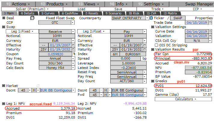
合约条款

对存续的利率互换合约进行估值，通常是根据当前的期限结构计算出浮动端（floating leg）和固定端（fixed leg）的“预期贴现现金流”，两者之差即合约的估值。需要注意的是，利率互换的估值对合约条款比较敏感。

示例中的合约是一个 Euribor 6M 的利率互换，条款细则如下：

• 浮动利率：Euribor 6M
• 固定利率：0.059820%
• 利差：0.0%
• 生效期：2007-01-19
• 期限：25 Y
• 类型：支付浮动利率，收取固定利率
• 浮动端支付频率：半年一次
• 浮动端天数计算规则：ACT/360
• 固定端支付频率：一年一次
• 固定端天数计算规则：30U/360
• 日历：TARGET（匹配 Trans-European Automated Real-time Gross Settlement Express Transfer System 的日历）
• 估值日期：2019-04-15

实践

import QuantLib as ql
import prettytable as pt

calendar = ql.TARGET()
evaluationDate = ql.Date(15, ql.April, 2019)
ql.Settings.instance().evaluationDate = evaluationDate

设置期限结构

估值的核心是当前的期限结构，根据 Real world tidy interest rate swap pricing 中的贴现因子数据设置估值用的期限结构。

Maturity Date	Discount Factors
04/15/2019	NA
04/23/2019	1.0000735
05/16/2019	1.0003059
07/16/2019	1.0007842
10/16/2019	1.0011807
04/16/2020	1.0023373
10/16/2020	1.0033115
04/16/2021	1.0039976
04/19/2022	1.0039393
04/17/2023	1.0015958
04/16/2024	0.9972325
04/16/2025	0.9907452
04/16/2026	0.9820912
04/16/2027	0.9715859
04/18/2028	0.9591332
04/16/2029	0.9455427
04/16/2030	0.9311096
04/16/2031	0.9161298
04/17/2034	0.8705738
04/18/2039	0.8017461
04/19/2044	0.7464983
04/20/2049	0.7010373
04/16/2054	0.6626670
04/16/2059	0.6289098
04/16/2064	0.5974307
04/16/2069	0.5684840

# discount curve

curveDates = [
    ql.Date(15, ql.April, 2019), ql.Date(23, ql.April, 2019), ql.Date(16, ql.May, 2019), ql.Date(16, ql.July, 2019),
    ql.Date(16, ql.October, 2019), ql.Date(16, ql.April, 2020), ql.Date(16, ql.October, 2020), ql.Date(16, ql.April, 2021),
    ql.Date(19, ql.April, 2022), ql.Date(17, ql.April, 2023), ql.Date(16, ql.April, 2024), ql.Date(16, ql.April, 2025),
    ql.Date(16, ql.April, 2026), ql.Date(16, ql.April, 2027), ql.Date(18, ql.April, 2028), ql.Date(16, ql.April, 2029),
    ql.Date(16, ql.April, 2030), ql.Date(16, ql.April, 2031), ql.Date(17, ql.April, 2034), ql.Date(18, ql.April, 2039),
    ql.Date(19, ql.April, 2044), ql.Date(20, ql.April, 2049), ql.Date(16, ql.April, 2054), ql.Date(16, ql.April, 2059),
    ql.Date(16, ql.April, 2064), ql.Date(16, ql.April, 2069)]

discountFactors = [
    1.0, 1.0000735, 1.0003059, 1.0007842, 1.0011807, 1.0023373, 1.0033115,
    1.0039976, 1.0039393, 1.0015958, 0.9972325, 0.9907452, 0.9820912, 0.9715859,
    0.9591332, 0.9455427, 0.9311096, 0.9161298, 0.8705738, 0.8017461, 0.7464983,
    0.7010373, 0.6626670, 0.6289098, 0.5974307, 0.5684840]

discountCurve = ql.DiscountCurve(
    curveDates,
    discountFactors,
    ql.Actual360(),  # 与浮动端一致
    calendar)

discountCurveHandle = ql.YieldTermStructureHandle(discountCurve)

添加历史浮动利率

估值利率互换需要用到一个重要的类——IborIndex，它负责根据期限结构以及合约的条款推算出隐含的远期利率，进而得到浮动端的预期现金流。

由于是对存续合约估值，需要为期限结构添加“历史浮动利率”——历史上 fixing date 上的 Euribor 6M 数据。尽管只有最近一次 fixing 的 Euribor 6M 利率会参与估值，但用户还是要添加更早期 fixing date 的利率，否则会报错，幸运的是它们不参与估值，可以用 0 来填充。

euriborIndex = ql.Euribor6M(discountCurveHandle)

# add fixing dates and rates for floating leg

unusedRate = 0.0  # not used in pricing
rate20190117 = -0.00236  # euribor-6M at 2019-01-17

euriborIndex.addFixing(fixingDate=ql.Date(17, ql.January, 2007), fixing=unusedRate)
euriborIndex.addFixing(fixingDate=ql.Date(17, ql.July, 2007), fixing=unusedRate)
euriborIndex.addFixing(fixingDate=ql.Date(17, ql.January, 2008), fixing=unusedRate)
euriborIndex.addFixing(fixingDate=ql.Date(17, ql.July, 2008), fixing=unusedRate)
euriborIndex.addFixing(fixingDate=ql.Date(15, ql.January, 2009), fixing=unusedRate)
euriborIndex.addFixing(fixingDate=ql.Date(16, ql.July, 2009), fixing=unusedRate)
euriborIndex.addFixing(fixingDate=ql.Date(15, ql.January, 2010), fixing=unusedRate)
euriborIndex.addFixing(fixingDate=ql.Date(15, ql.July, 2010), fixing=unusedRate)
euriborIndex.addFixing(fixingDate=ql.Date(17, ql.January, 2011), fixing=unusedRate)
euriborIndex.addFixing(fixingDate=ql.Date(15, ql.July, 2011), fixing=unusedRate)
euriborIndex.addFixing(fixingDate=ql.Date(17, ql.January, 2012), fixing=unusedRate)
euriborIndex.addFixing(fixingDate=ql.Date(17, ql.July, 2012), fixing=unusedRate)
euriborIndex.addFixing(fixingDate=ql.Date(17, ql.January, 2013), fixing=unusedRate)
euriborIndex.addFixing(fixingDate=ql.Date(17, ql.July, 2013), fixing=unusedRate)
euriborIndex.addFixing(fixingDate=ql.Date(16, ql.January, 2014), fixing=unusedRate)
euriborIndex.addFixing(fixingDate=ql.Date(17, ql.July, 2014), fixing=unusedRate)
euriborIndex.addFixing(fixingDate=ql.Date(15, ql.January, 2015), fixing=unusedRate)
euriborIndex.addFixing(fixingDate=ql.Date(16, ql.July, 2015), fixing=unusedRate)
euriborIndex.addFixing(fixingDate=ql.Date(15, ql.January, 2016), fixing=unusedRate)
euriborIndex.addFixing(fixingDate=ql.Date(15, ql.July, 2016), fixing=unusedRate)
euriborIndex.addFixing(fixingDate=ql.Date(17, ql.January, 2017), fixing=unusedRate)
euriborIndex.addFixing(fixingDate=ql.Date(17, ql.July, 2017), fixing=unusedRate)
euriborIndex.addFixing(fixingDate=ql.Date(17, ql.January, 2018), fixing=unusedRate)
euriborIndex.addFixing(fixingDate=ql.Date(17, ql.July, 2018), fixing=unusedRate)
euriborIndex.addFixing(fixingDate=ql.Date(17, ql.January, 2019), fixing=rate20190117)

注：Euribor6M 是 IborIndex 的派生类。

设置合约

一些基本设置：

# swap contrast

nominal = 10000000.0
spread = 0.0
swapType = ql.VanillaSwap.Receiver
lengthInYears = 25
effectiveDate = ql.Date(19, ql.January, 2007)
terminationDate = effectiveDate + ql.Period(lengthInYears, ql.Years)

设置固定端与浮动端的支付时间表（schedule），计算出现金流的发生日期：

# fixed leg

fixedLegFrequency = ql.Period(ql.Annual)
fixedLegConvention = ql.ModifiedFollowing
fixedLegDayCounter = ql.Thirty360(ql.Thirty360.USA)
fixedDateGeneration = ql.DateGeneration.Forward
fixedRate = 0.059820 / 100.0

fixedSchedule = ql.Schedule(
    effectiveDate,
    terminationDate,
    fixedLegFrequency,
    calendar,
    fixedLegConvention,
    fixedLegConvention,
    fixedDateGeneration,
    False)

# floating leg

floatingLegFrequency = ql.Period(ql.Semiannual)
floatingLegConvention = ql.ModifiedFollowing
floatingLegDayCounter = ql.Actual360()
floatingDateGeneration = ql.DateGeneration.Forward

floatSchedule = ql.Schedule(
    effectiveDate,
    terminationDate,
    floatingLegFrequency,
    calendar,
    floatingLegConvention,
    floatingLegConvention,
    floatingDateGeneration,
    False)

VanillaSwap 类实现了普通利率互换，VanillaSwap 类将接受一个定价引擎——DiscountingSwapEngine，并根据前面配置好的现金流日期计算浮动端和固定端的预期贴现现金流。

spot25YearSwap = ql.VanillaSwap(
    swapType,
    nominal,
    fixedSchedule,
    fixedRate,
    fixedLegDayCounter,
    floatSchedule,
    euriborIndex,
    spread,
    floatingLegDayCounter)

swapEngine = ql.DiscountingSwapEngine(discountCurveHandle)
spot25YearSwap.setPricingEngine(swapEngine)

估值

Bloomberg 对浮动端和固定端的估值考虑了本金，而 QuantLib 默认不考虑本金，所以浮动端和固定端的 NPV 要自己计算。

fixedNpv = 0.0
floatingNpv = 0.0

fixedTable = pt.PrettyTable(['date', 'amount'])

for cf in spot25YearSwap.fixedLeg():
    if cf.date() > evaluationDate:
        fixedTable.add_row([str(cf.date()), cf.amount()])
        fixedNpv = fixedNpv + discountCurveHandle.discount(cf.date()) * cf.amount()

fixedNpv = fixedNpv + discountCurveHandle.discount(
    spot25YearSwap.fixedLeg()[-1].date()) * nominal

floatingTable = pt.PrettyTable(['date', 'amount'])

for cf in spot25YearSwap.floatingLeg():
    if cf.date() > evaluationDate:
        floatingTable.add_row([str(cf.date()), cf.amount()])
        floatingNpv = floatingNpv + discountCurveHandle.discount(cf.date()) * cf.amount()

floatingNpv = floatingNpv + discountCurveHandle.discount(
    spot25YearSwap.floatingLeg()[-1].date()) * nominal

npvTable = pt.PrettyTable(['NPVs', 'amount'])
npvTable.add_row(['total', spot25YearSwap.NPV()])
npvTable.add_row(['fixed leg NPV', fixedNpv])
npvTable.add_row(['floating leg NPV', floatingNpv])

npvTable.align = 'r'
npvTable.float_format = '.2'
print('NPVs:')
print(npvTable)
print()

fixedTable.align = 'r'
fixedTable.float_format = '.4'
print('Fixed Leg Cash Flows (no nominal):')
print(fixedTable)
print()

floatingTable.align = 'r'
floatingTable.float_format = '.4'
print('Floating Leg Cash Flows (no nominal):')
print(floatingTable)

结果：

NPVs:
+------------------+------------+
|             NPVs |     amount |
+------------------+------------+
|            total | -877065.26 |
|    fixed leg NPV | 9119162.21 |
| floating leg NPV | 9996227.47 |
+------------------+------------+

Fixed Leg Cash Flows (no nominal):
+--------------------+-----------+
|               date |    amount |
+--------------------+-----------+
| January 20th, 2020 | 5965.3833 |
| January 19th, 2021 | 5965.3833 |
| January 19th, 2022 | 5982.0000 |
| January 19th, 2023 | 5982.0000 |
| January 19th, 2024 | 5982.0000 |
| January 20th, 2025 | 5998.6167 |
| January 19th, 2026 | 5965.3833 |
| January 19th, 2027 | 5982.0000 |
| January 19th, 2028 | 5982.0000 |
| January 19th, 2029 | 5982.0000 |
| January 21st, 2030 | 6015.2333 |
| January 20th, 2031 | 5965.3833 |
| January 19th, 2032 | 5965.3833 |
+--------------------+-----------+

Floating Leg Cash Flows (no nominal):
+--------------------+-------------+
|               date |      amount |
+--------------------+-------------+
|    July 19th, 2019 | -11734.4444 |
| January 20th, 2020 |  -9883.8108 |
|    July 20th, 2020 | -10526.4706 |
| January 19th, 2021 |  -8236.3411 |
|    July 19th, 2021 |  -3118.9504 |
| January 19th, 2022 |    290.3520 |
|    July 19th, 2022 |   6002.4970 |
| January 19th, 2023 |  11853.1381 |
|    July 19th, 2023 |  16803.6213 |
| January 19th, 2024 |  22032.9795 |
|    July 19th, 2024 |  27371.4264 |
| January 20th, 2025 |  33134.5740 |
|    July 21st, 2025 |  38526.4090 |
| January 19th, 2026 |  43841.7013 |
|    July 20th, 2026 |  49022.3996 |
| January 19th, 2027 |  54065.4048 |
|    July 19th, 2027 |  58756.3184 |
| January 19th, 2028 |  64707.0763 |
|    July 19th, 2028 |  67946.7395 |
| January 19th, 2029 |  72599.6699 |
|    July 19th, 2029 |  74090.1906 |
| January 21st, 2030 |  78693.2841 |
|    July 19th, 2030 |  77892.3324 |
| January 20th, 2031 |  82544.3792 |
|    July 21st, 2031 |  83194.2799 |
| January 19th, 2032 |  84980.7972 |
+--------------------+-------------+

估值差异可能的来源

与 Bloomberg 的结果相比尽管非常接近，但还是存在差异，估值差异的来源可能如下：

• 在期限结构上插值的技术细节不一致。DiscountCurve 对贴现因子进行对数线性插值，Bloomberg 的技术细节不得而知。
• 浮动端和固定端的天数计算规则不一致，而期限结构的天数计算规则与浮动端保持一致。天数计算规则的不一致使得同一“日期”对浮动端和固定端来说意味着不同的“时间”，Bloomberg 如何处理这种不一致也不得而知。

下一步

• 分析国内市场上的利率互换。
• 从利率互换的成交报价中推算期限结构。