壁虎书7 Ensemble Learning and Random Forests

　　if you aggregate the predictions of a group of predictors，you will often get better predictions than with the best individual predictor. a group of predictors is called an ensemble；this technique is called Ensemble Learning，and an Ensemble Learning algorithm is called an Ensemble method. 

　　for example，you can train a group of Decision Tree classifiers，each on a different random subset of the training set. to make predictions，you just obtain the predictions of all individual trees，then predict the class that gets the most votes. such an ensemble of Decision Trees is called a Random Forest，and despite its simplicity，this is one of the most powerful Machine Learning algorithms available today. 

　　moreover，you will often use Ensemble methods near the end of a project，once you have already built a few good predictors，to combine them into an even better predictor. 

　　the most popular Ensemble methods，including bagging，boosting，stacking，Random Forests. 

Voting Classifiers: 

　　Suppose you have trained a few classifiers, each one achieving about 80% accuracy. You may have a Logistic Regression classifier, an SVM classifier, a Random Forest classifier, a K-Nearest Neighbors classifier, and perhaps a few more (see Figure 7-1)

　　

　　A very simple way to create an even better classifier is to aggregate the predictions of each classifier and predict the class that gets the most votes. This majority-vote classifier is called a hard voting classifier (see Figure 7-2). 

　　

　　Somewhat surprisingly, this voting classifier often achieves a higher accuracy than the best classifier in the ensemble. In fact, even if each classifier is a weak learner (meaning it does only slightly better than random guessing), the ensemble can still be a strong learner (achieving high accuracy), provided there are a sufficient number of weak learners and they are sufficiently diverse. 

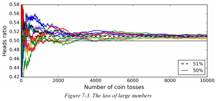
　　How is this possible? The following analogy can help shed some light on this mystery. Suppose you have a slightly biased coin that has a 51% chance of coming up heads, and 49% chance of coming up tails. If you toss it 1,000 times, you will generally get more or less 510 heads and 490 tails, and hence a majority of heads. If you do the math, you will find that the probability of obtaining a majority of heads after 1,000 tosses is close to 75%. The more you toss the coin, the higher the probability (e.g., with 10,000 tosses, the probability climbs over 97%). This is due to the law of large numbers: as you keep tossing the coin, the ratio of heads gets closer and closer to the probability of heads (51%). 

　　Similarly, suppose you build an ensemble containing 1,000 classifiers that are individually correct only 51% of the time (barely better than random guessing). If you predict the majority voted class, you can hope for up to 75% accuracy! However, this is only true if all classifiers are perfectly independent, making uncorrelated errors, which is clearly not the case since they are trained on the same data. They are likely to make the same types of errors, so there will be many majority votes for the wrong class, reducing the ensemble’s accuracy. 

　　Figure 7-3 shows 10 series of biased coin tosses. You can see that as the number of tosses increases, the ratio of headsapproaches 51%. Eventually all 10 series end up so close to 51% that they are consistently above 50%. 

import numpy as np
import matplotlib.pyplot as plt

heads_proba = 0.51
coin_tosses = (np.random.rand(10000, 10) < heads_proba).astype(np.int32)
cumulative_heads_ratio = np.cumsum(coin_tosses, axis=0) / np.arange(1, 10001).reshape(-1, 1)

plt.figure(figsize=(8, 3.5))
plt.plot(cumulative_heads_ratio)
plt.plot([0, 10000], [0.51, 0.51], "k--", linewidth=2, label="51%")
plt.plot([0, 10000], [0.5, 0.5], "k-", label="50%")
plt.xlabel("Number of coin tosses")
plt.ylabel("Heads ratio")
plt.legend(loc="lower right")
plt.axis([0, 10000, 0.42, 0.58])
plt.show()

　　

from sklearn.datasets import make_moons
from sklearn.model_selection import train_test_split
from sklearn.linear_model import LogisticRegression
from sklearn.ensemble import RandomForestClassifier, VotingClassifier
from sklearn.svm import SVC
from sklearn.metrics import accuracy_score

X, y = make_moons(n_samples=500, noise=0.30, random_state=42)
X_train, X_test, y_train, y_test = train_test_split(X, y, random_state=42)

log_clf = LogisticRegression(solver='liblinear', random_state=42)
rnd_clf = RandomForestClassifier(n_estimators=10, random_state=42)
svm_clf = SVC(gamma='auto', random_state=42)

voting_clf = VotingClassifier(
    estimators=[('lr', log_clf), ('rf', rnd_clf), ('svc', svm_clf)],
    voting='hard'
)
voting_clf.fit(X_train, y_train)

for clf in (log_clf, rnd_clf, svm_clf, voting_clf):
    clf.fit(X_train, y_train)
    y_pred = clf.predict(X_test)
    print(clf.__class__.__name__, accuracy_score(y_test, y_pred))

# LogisticRegression 0.864
# RandomForestClassifier 0.872
# SVC 0.888
# VotingClassifier 0.896

　　if all classifiers are able to estimate class probabilities (i.e., they have a predict_proba() method)，then you can tell Scikit-Learn to predict the class with the highest class probability，averaged over all the individual classifiers. this is called soft voting. it often achieves higher performance than hard voting because it gives more weight to highly confident votes. 

　　All you need to do is replace voting="hard" with voting="soft" and ensure that all classifiers can estimate class probabilities. This is not the case of the SVC class by default, so you need to set its probability hyperparameter to True (this will make the SVC class use cross-validation to estimate class probabilities, slowing down training, and it will add a predict_proba() method).

X, y = make_moons(n_samples=500, noise=0.30, random_state=42)
X_train, X_test, y_train, y_test = train_test_split(X, y, random_state=42)

log_clf = LogisticRegression(solver='liblinear', random_state=42)
rnd_clf = RandomForestClassifier(n_estimators=10, random_state=42)
svm_clf = SVC(gamma='auto', probability=True, random_state=42)  # voting='soft'时，predict_proba必须可用。

voting_clf = VotingClassifier(
    estimators=[('lr', log_clf), ('rf', rnd_clf), ('svc', svm_clf)],
    voting='soft'
)
voting_clf.fit(X_train, y_train)

for clf in (log_clf, rnd_clf, svm_clf, voting_clf):
    clf.fit(X_train, y_train)
    y_pred = clf.predict(X_test)
    print(clf.__class__.__name__, accuracy_score(y_test, y_pred))

# LogisticRegression 0.864
# RandomForestClassifier 0.872
# SVC 0.888
# VotingClassifier 0.912

Bagging and Pasting: 

　　Bagging and Pasting in Scikit-Learn

　　Out-of-Bag Evaluation

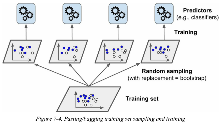
　　one way to get a diverse set of classifiers is to use very different training algorithms. another approach is to use the same training algorithm for every predictor，but to train them on different random subsets of the training set. when sampling is performed with replacement，this method is called bagging(short for bootstrap aggregating). when sampling is performed without replacement，it is called pasting. 

　　once all predictors are trained，the ensemble can make a prediction for a new instance by simply aggregating the predictions of all predictors. the aggregating function is typically the statistical mode for classification，or the average for regression. 

　　each individual predictor has a higher bias than if it were trained on the original training set，but aggregation reduces both bias and variance. generally，the net result is that the ensemble has a similar bias but a lower variance than a single predictor trained on the original training set. 

　　as you can see in Figure 7-4，predictors can all be trained in parallel，via different CPU cores or even different servers. similarly，predictions can be made in parallel. this is one of the reasons why bagging and pasting are such popular methods: they scale very well. 

　　

Bagging and Pasting in Scikit-Learn: 

　　Scikit-Learn offers a simple API for both bagging and pasting with the BaggingClassifier and BaggingRegression.

　　the following code trains an ensemble of 500 Decision Tree classifiers，each trained on 100 training instances randomly sampled from the training set with replacement(bagging if bootstrap=True else pasting).  the n_jobs parameter tells Scikit-Learn the number of CPU cores to use for training and predictions(-1 tells Scikit-Learn to use all available cores)

from sklearn.datasets import make_moons
from sklearn.model_selection import train_test_split
from sklearn.ensemble import BaggingClassifier
from sklearn.tree import DecisionTreeClassifier
from sklearn.metrics import accuracy_score

X, y = make_moons(n_samples=500, noise=0.30, random_state=42)
X_train, X_test, y_train, y_test = train_test_split(X, y, random_state=42)

bag_clf = BaggingClassifier(
    base_estimator=DecisionTreeClassifier(random_state=42), n_estimators=500,
    max_samples=100, bootstrap=True, n_jobs=-1, random_state=42
)
bag_clf.fit(X_train, y_train)

y_pred = bag_clf.predict(X_test)
print(accuracy_score(y_test, y_pred))  # 0.904

　　note: the BaggingClassifier automatically performs soft voting instead of hard voting if the base classifier can estimate class probabilities，which is the case with Decision Trees classifiers. 

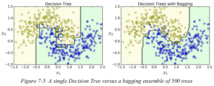
　　Figure 7-5 compares the decision boundary of a single Decision Tree with the decision boundary of a bagging ensemble of 500 trees, both trained on the moons dataset. As you can see, the ensemble’s predictions will likely generalize much better than the single Decision Tree’s predictions: the ensemble has a comparable bias but a smaller variance (it makes roughly the same number of errors on the training set, but the decision boundary is less irregular). 

　　

　　bootstrapping introduces a bit more diversity in the subsets that each predictor is trained on，so bagging ends up with a slightly higher bias than pasting，but this also means that predictors end up being less correlated so the ensemble's variance is reduced. overall，bagging often results in better models，which explained why it is generally preferred. 

Out-of-Bag Evaluation: 

　　With bagging, some instances may be sampled several times for any given predictor, while others may not be sampled at all. By default a BaggingClassifier samples m training instances with replacement ( bootstrap=True ), where m is the size of the training set. This means that only about 63% of the training instances are sampled on average for each predictor. The remaining 37% of the training instances that are not sampled are called out-of-bag (oob) instances. Note that they are not the same 37% for all predictors.

　　Since a predictor never sees the oob instances during training, it can be evaluated on these instances, without the need for a separate validation set or cross-validation. You can evaluate the ensemble itself by averaging out the oob evaluations of each predictor. 

　　In Scikit-Learn, you can set oob_score=True when creating a BaggingClassifier to request an automatic oob evaluation after training. The following code demonstrates this. The resulting evaluation score is available through the oob_score_ variable: 

　　the oob decision function for each training instance is also available through the oob_decision_function_ variable. in this case (since the base estimator has a predict_proba() method) the decision function returns the class probabilities for each training instance. 

from sklearn.datasets import make_moons
from sklearn.model_selection import train_test_split
from sklearn.ensemble import BaggingClassifier
from sklearn.tree import DecisionTreeClassifier
from sklearn.metrics import accuracy_score

X, y = make_moons(n_samples=500, noise=0.30, random_state=42)
X_train, X_test, y_train, y_test = train_test_split(X, y, random_state=42)

bag_clf = BaggingClassifier(
    base_estimator=DecisionTreeClassifier(random_state=42), n_estimators=500,
    bootstrap=True, n_jobs=-1, random_state=40,
    oob_score=True
)
bag_clf.fit(X_train, y_train)

print(bag_clf.oob_score_)  # 0.9013333333333333
print(bag_clf.oob_decision_function_)

y_pred = bag_clf.predict(X_test)
print(accuracy_score(y_test, y_pred))  # 0.912

Random Patches and Random Subspaces: 

　　The BaggingClassifier class supports sampling the features as well. This is controlled by two hyperparameters: max_features and bootstrap_features. They work the same way as max_samples and bootstrap, but for feature sampling instead of instance sampling. Thus, each predictor will be trained on a random subset of the input features. 

　　This is particularly useful when you are dealing with high-dimensional inputs (such as images).

　　Sampling both training instances and features is called the Random Patches method.

　　Keeping all training instances (i.e., bootstrap=False and max_samples=1.0 ) but sampling features (i.e., bootstrap_features=True and/or max_features smaller than 1.0) is called the Random Subspaces method. 

　　Sampling features results in even more predictor diversity, trading a bit more bias for a lower variance. 

Random Forests: 

　　Extra-Trees

　　Feature Importance

　　as we have discussed，a Random Forest is an ensemble of Decision Trees，generally trained via the bagging method (or sometimes pasting)，typically with max_samples set to the training set. instead of building a BaggingClassifier and passing it a DecisionTreeClassifier，you can instead use the RandomForestClassifier/ RandomForestRegressor class，which is more convenient and optimized for Decision Trees. 

　　With a few exceptions, a RandomForestClassifier has all the hyperparameters of a DecisionTreeClassifier (to control how trees are grown), plus all the hyperparameters of a BaggingClassifier to control the ensemble itself. 

　　The Random Forest algorithm introduces extra randomness when growing trees；instead of searching for the very best feature when splitting a node, it searches for the best feature among a random subset of features. This results in a greater tree diversity, which (once again) trades a higher bias for a lower variance, generally yielding an overall better model. The following BaggingClassifier is roughly equivalent to the previous RandomForestClassifier :

import numpy as np
from sklearn.datasets import make_moons
from sklearn.model_selection import train_test_split
from sklearn.ensemble import BaggingClassifier
from sklearn.tree import DecisionTreeClassifier
from sklearn.ensemble import RandomForestClassifier
from sklearn.metrics import accuracy_score

X, y = make_moons(n_samples=500, noise=0.30, random_state=42)
X_train, X_test, y_train, y_test = train_test_split(X, y, random_state=42)

bag_clf = BaggingClassifier(
    base_estimator=DecisionTreeClassifier(splitter='random', max_leaf_nodes=16, random_state=42), n_estimators=500,
    n_jobs=-1, random_state=42,
)
rnd_clf = RandomForestClassifier(n_estimators=500, n_jobs=-1, max_leaf_nodes=16, random_state=42)
bag_clf.fit(X_train, y_train)
rnd_clf.fit(X_train, y_train)

y_pred = bag_clf.predict(X_test)
print(accuracy_score(y_test, y_pred))  # 0.92

y_pred_rf = rnd_clf.predict(X_test)
print(accuracy_score(y_test, y_pred_rf))  # 0.912

print(np.sum(y_pred == y_pred_rf) / len(y_pred))  # 0.976

Extra-Trees: 

　　when you are growing a tree in a Random Forest，at each node only a random subset of the features is considered for splitting. it is possible to make trees even more random by also using random thresholds for each feature rather than searching for the best possible thresholds. 

　　A forest of such extremely random trees is simply called an Extremely Randomized Trees ensemble (or Extra-Trees for short). Once again, this trades more bias for a lower variance. It also makes Extra-Trees much faster to train than regular Random Forests since finding the best possible threshold for each feature at every node is one of the most time-consuming tasks of growing a tree. 
　　You can create an Extra-Trees classifier using Scikit-Learn’s ExtraTreesClassifier class. Its API is identical to the RandomForestClassifier class. Similarly, the ExtraTreesRegressor class has the same API as the RandomForestRegressor class. 

　　tip: It is hard to tell in advance whether a RandomForestClassifier will perform better or worse than an ExtraTreesClassifier. Generally, the only way to know is to try both and compare them using cross-validation (and tuning the hyperparameters using grid search). 

Featuer Importance: 

　　Lastly, if you look at a single Decision Tree, important features are likely to appear closer to the root of the tree, while unimportant features will often appear closer to the leaves (or not at all). It is therefore possible to get an estimate of a feature’s importance by computing the average depth at which it appears across all trees in the forest. Scikit-Learn computes this automatically for every feature after training. You can access the result using the feature_importances_ variable. For example, the following code trains a RandomForestClassifier on the iris dataset and outputs each feature’s importance. It seems that the most important features are the petal length (44%) and width (42%), while sepal length and width are rather unimportant in comparison (11% and 2%, respectively):

　　以 moon 数据为例，

from sklearn.ensemble import RandomForestClassifier
from sklearn.datasets import load_iris

iris = load_iris()

rnd_clf = RandomForestClassifier(n_estimators=500, n_jobs=-1, random_state=42)
rnd_clf.fit(iris['data'], iris['target'])

for name, score in zip(iris['feature_names'], rnd_clf.feature_importances_):
    print(name, score)

# sepal length (cm) 0.11249225099876374
# sepal width (cm) 0.023119288282510326
# petal length (cm) 0.44103046436395765
# petal width (cm) 0.4233579963547681

　　以 mnist 数据为例，

import numpy as np
import matplotlib.pyplot as plt
from sklearn.ensemble import RandomForestClassifier
from sklearn.datasets import fetch_openml

mnist = fetch_openml('mnist_784', version=1)
mnist.target = mnist.target.astype(np.int64)

rnd_clf = RandomForestClassifier(n_estimators=10, n_jobs=-1, random_state=42)
rnd_clf.fit(mnist['data'], mnist['target'])


def plot_digit(data):
    image = data.reshape(28, 28)
    plt.imshow(image, cmap=plt.cm.hot, interpolation='nearest')
    plt.axis('off')


plot_digit(rnd_clf.feature_importances_)
cbar = plt.colorbar(ticks=[rnd_clf.feature_importances_.min(), rnd_clf.feature_importances_.max()])
cbar.ax.set_yticklabels(['Not important', 'Very important'])
plt.show()

　　 

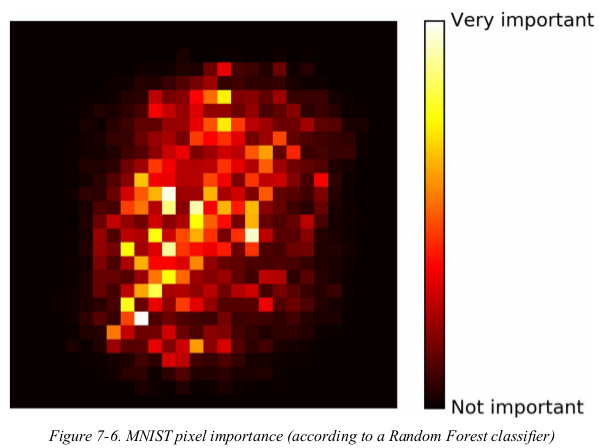
　　Random Forests are very handy to get a quick understanding of what features actually matter，in particular if you need to perform feature selection. 

Boosting: 

　　AdaBoost

　　Gradient Boosting

　　Boosting refers to any ensemble method that can combine several weak learners into a strong learner. the general idea of most boosting methods is to train predictors sequentially，each trying to correct its predecessor. by far the most popular are AdaBoost (short for Adaptive Boosting) and Gradient Boosting. 

AdaBoost: 

　　one way for a new predictor to correct its predecessor is to pay a bit more attention to the training instances that the predecessor underfitted. this results in new predictors focusing more and more on the hard cases. this is the technique used by AdaBoost. 

　　For example, to build an AdaBoost classifier, a first base classifier (such as a Decision Tree) is trained and used to make predictions on the training set. The relative weight of misclassified training instances is then increased. A second classifier is trained using the updated weights and again it makes predictions on the training set, weights are updated, and so on (see Figure 7-7). 

　　

　　

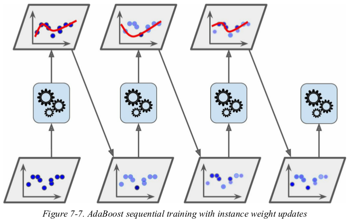
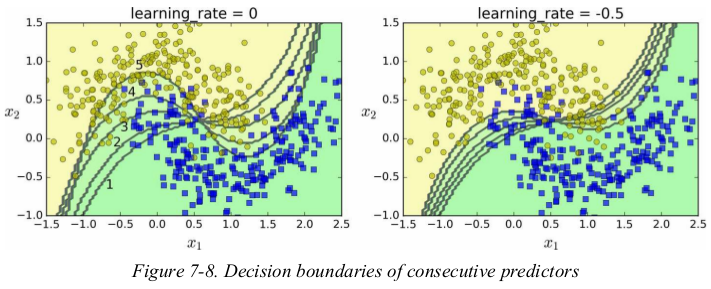
　　Figure 7-8 shows the decision boundaries of five consecutive predictors on the moons dataset (in this example, each predictor is a highly regularized SVM classifier with an RBF kernel ). The first classifier gets many instances wrong, so their weights get boosted. The second classifier therefore does a better job on these instances, and so on. The plot on the right represents the same sequence of predictors except that the learning rate is halved (i.e., the misclassified instance weights are boosted half as much at every iteration). As you can see, this sequential learning technique has some similarities with Gradient Descent, except that instead of tweaking a single predictor’s parameters to minimize a cost function, AdaBoost adds predictors to the ensemble, gradually making it better. 

import numpy as np
import matplotlib.pyplot as plt
from sklearn.model_selection import train_test_split
from sklearn.datasets import make_moons
from sklearn.svm import SVC

X, y = make_moons(n_samples=500, noise=0.30, random_state=42)
X_train, X_test, y_train, y_test = train_test_split(X, y, random_state=42)


m = len(X_train)
plt.figure(figsize=(11, 4))
for subplot, learning_rate in ((121, 1), (122, 0.5)):
    sample_weghts = np.ones(m)
    plt.subplot(subplot)
    for i in range(5):
        svm_clf = SVC(C=0.05, gamma='auto', random_state=42)
        svm_clf.fit(X_train, y_train, sample_weight=sample_weghts)
        y_pred = svm_clf.predict(X_train)
        sample_weghts[y_pred != y_train] *= (1 + learning_rate)  # 更新样例的权重
        plot_decision_boundary(svm_clf, X, y, alpha=0.2)
    plt.title('learning_rate = {}'.format(learning_rate), fontsize=16)

plt.show()

　　

看到这里可以知道，Bagging and Pasting 是针对样本和特征的，Boosting是针对模型的。

　　there is one important drawback to this sequential learning technique: it can't be parallelized，since each predictor can only be trained after the previous predictor has been trained and evaluated. as a result，it doesn't scale as well as bagging or pasting. 

　　

　　let’s take a closer look at the AdaBoost algorithm.

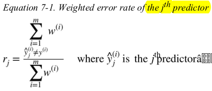
　　Each instance weight w⁽ⁱ⁾ is initially set to 1/m. A first predictor is trained and its weighted error rate r₁ is computed on the training set；see Equation 7-1. 

　　

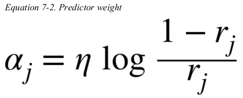
　　The predictor’s weight α_j is then computed using Equation 7-2，where η is the learning rate hyperparameter (defaults to 1). The more accurate the predictor is，the higher its weight will be. If it is just guessing randomly，then its weight will be close to zero. However，if it is most often wrong (i.e., less accurate than random guessing), then its weight will be negative.

　　

　　Next the instance weights are updated using Equation 7-3: the misclassified instances are boosted.

　　

　　如果一个predictor 的预测值大半都是错误的，那么a_j就为负，错误实例的权重减小；如果一个predictor 的预测值只有少数错误，那么a_j为正，错误实例的权重增加。

　　Then all the instance weights are normalized (i.e., divided by). 

　　Finally，a new predictor is trained using the updated weights，and the whole process is repeated. The algorithm stops when the desired number of predictors is reached, or when a perfect predictor is found. 

　　

　　To make predictions，AdaBoost simply computes the predictions of all the predictors and weighs them using the predictor weights α _j. The predicted class is the one that receives the majority of weighted votes (see Equation 7-4). 

　　

　　

　　Scikit-Learn actually uses a multiclass version of AdaBoost called SAMME (which stands for Stagewise Additive Modeling using a Multiclass Exponential loss function). When there are just two classes，SAMME is equivalent to AdaBoost. Moreover，if the predictors can estimate class probabilities (i.e., if they have a predict_proba() method)，Scikit-Learn can use a variant of SAMME called SAMME.R (the R stands for “Real”)，which relies on class probabilities rather than predictions and generally performs better. 

　　The following code trains an AdaBoost classifier based on 200 Decision Stumps using Scikit-Learn’s AdaBoostClassifier class (as you might expect，there is also an AdaBoostRegressor class). A Decision Stump is a Decision Tree with max_depth=1 — in other words，a tree composed of a single decision node plus two leaf nodes. This is the default base estimator for the AdaBoostClassifier class:

from sklearn.model_selection import train_test_split
from sklearn.tree import DecisionTreeClassifier
from sklearn.ensemble import AdaBoostClassifier, AdaBoostRegressor
from sklearn.datasets import make_moons

X, y = make_moons(n_samples=500, noise=0.30, random_state=42)
X_train, X_test, y_train, y_test = train_test_split(X, y, random_state=42)

ada_clf = AdaBoostClassifier(
    base_estimator=DecisionTreeClassifier(max_depth=1), n_estimators=200,
    learning_rate=0.5, algorithm='SAMME.R', random_state=42
)
ada_clf.fit(X_train, y_train)

　　

　　If your AdaBoost ensemble is overfitting the training set，you can try reducing the number of estimators or more strongly regularizing the base estimator. 

Gradient Boosting: 

　　Just like AdaBoost，Gradient Boosting works by sequentially adding predictors to an ensemble，each one correcting its predecessor. However，instead of tweaking the instance weights at every iteration like AdaBoost does，this method tries to fit the new predictor to the residual errors made by the previous predictor.

　　Let’s go through a simple regression example using Decision Trees as the base predictors. This is called Gradient Tree Boosting，or Gradient Boosted Regression Trees (GBRT). 

import numpy as np
import matplotlib.pyplot as plt
from sklearn.tree import DecisionTreeRegressor

np.random.seed(42)
X = np.random.rand(100, 1) - 0.5
y = 3*X[:, 0]**2 + 0.05 * np.random.randn(100)

tree_reg1 = DecisionTreeRegressor(max_depth=2)
tree_reg1.fit(X, y)

y2 = y - tree_reg1.predict(X)
tree_reg2 = DecisionTreeRegressor(max_depth=2)
tree_reg2.fit(X, y2)

y3 = y2 - tree_reg2.predict(X)
tree_reg3 = DecisionTreeRegressor(max_depth=2)
tree_reg3.fit(X, y3)

X_new = np.array([[0.8]])
y_pred = sum(tree.predict(X_new) for tree in (tree_reg1, tree_reg2, tree_reg3))
print(y_pred)  # [0.75026781]


def plot_predictions(regressors, X, y, axes=[-0.5, 0.5, -0.1, 0.8], label=None, style='r-', data_style='b.', data_label=None):
    # 画曲线用的并不是用的训练数据X，而是测试数据x1，x1是有序数据，X是无序数据，用X画图会生成一团线。
    x1 = np.linspace(axes[0], axes[1], 500)
    y_pred = sum(regressor.predict(x1.reshape(-1, 1)) for regressor in regressors)

    plt.plot(X, y, data_style, label=data_label)
    plt.plot(x1, y_pred, style, linewidth=2, label=label)
    if label or data_label:
        plt.legend(loc='upper center', fontsize=16)
    plt.axis(axes)


plt.figure(figsize=(11, 11))
plt.subplot(321)
plot_predictions([tree_reg1], X, y, label='$h_1(x_1)$', style='g-', data_label='Training set')
plt.ylabel('$y$', fontsize=16, rotation=0)
plt.title('Residuals and tree predictions', fontsize=16)
plt.subplot(322)
plot_predictions([tree_reg1], X, y, label='$h(x_1) = h_1(x_1)$', data_label='Training set')
plt.ylabel('$y$', fontsize=16, rotation=0)
plt.title('Ensemble predictions', fontsize=16)
plt.subplot(323)
plot_predictions([tree_reg2], X, y2, axes=[-0.5, 0.5, -0.5, 0.5], label='$h_2(x_1)$', style='g-', data_style='k+', data_label='Residuals')
plt.ylabel('$y - h_1(x_1)$', fontsize=16)
plt.subplot(324)
plot_predictions([tree_reg1, tree_reg2], X, y, label='$h(x_1) = h_1(x_1) + h_2(x_1)$')
plt.ylabel('$y$', fontsize=16, rotation=0)
plt.subplot(325)
plot_predictions([tree_reg3], X, y3, axes=[-0.5, 0.5, -0.5, 0.5], label='$h_3(x_1)$', style='g-', data_style='k+')
plt.ylabel('$y - h_1(x_1) - h_2(x_1)$', fontsize=16)
plt.xlabel('$x_1$', fontsize=16)
plt.subplot(326)
plot_predictions([tree_reg1, tree_reg2, tree_reg3], X, y, label='$h(x_1) = h_1(x_1) + h_2(x_1) + h_3(x_1)$')
plt.ylabel('$y$', fontsize=16, rotation=0)
plt.xlabel('$x_1$', fontsize=16)
plt.show()

　　

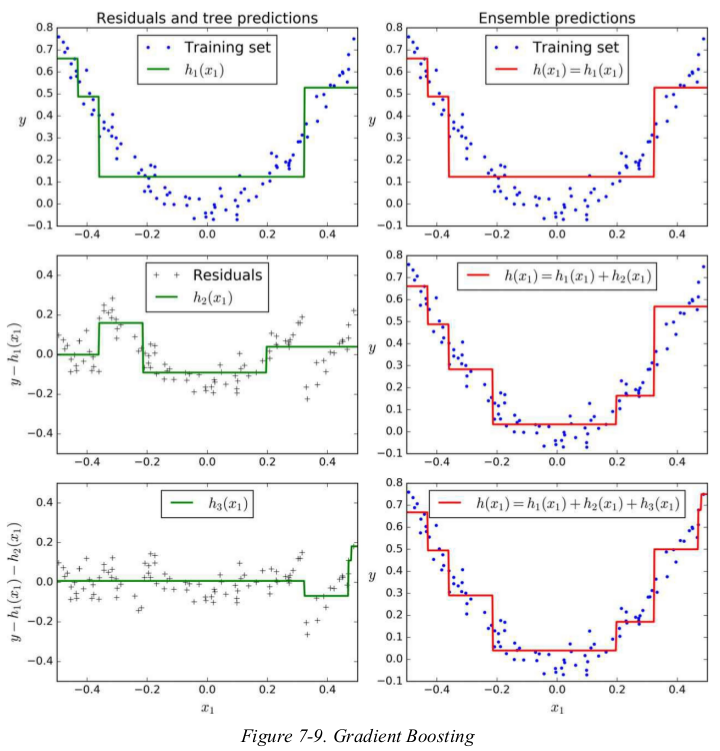
　　 上述: it can make predictions on a new instance simply by adding up the predictions of all predictors.

　　

　　a simpler way to train GBRT ensembles is to use Scikit-Learn's GradientBoostingRegressor class. Much like the RandomForestRegressorclass, it has hyperparameters to control the growth of Decision Trees (e.g., max_depth , min_samples_leaf , and so on), as well as hyperparameters to control the ensemble training, such as the number of trees ( n_estimators ). The following code creates the same ensemble as the previous one: 

from sklearn.ensemble import GradientBoostingRegressor

np.random.seed(42)
X = np.random.rand(100, 1) - 0.5
y = 3*X[:, 0]**2 + 0.05 * np.random.randn(100)

X_new = np.array([[0.8]])

gbrt = GradientBoostingRegressor(learning_rate=1.0, n_estimators=3, max_depth=2)
gbrt.fit(X, y)
print(gbrt.predict(X_new))  # [0.75026781]

　　The learning_rate hyperparameter scales the contribution of each tree. If you set it to a low value, such as 0.1 , you will need more trees in the ensemble to fit the training set, but the predictions will usually generalize better. This is a regularization technique called shrinkage.

　　Figure 7-10 shows two GBRT ensembles trained with a low learning rate: the one on the left does not have enough trees to fit the training set, while the one on the right has too many trees and overfits the training set. 

　　

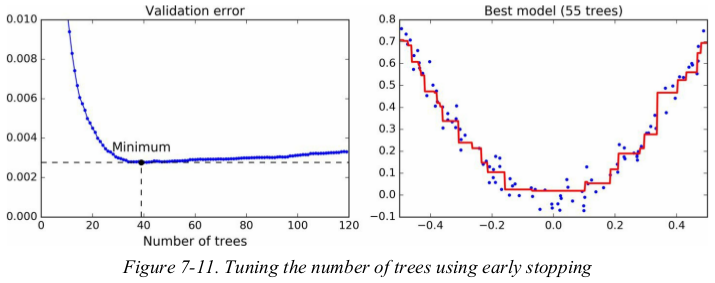
　　In order to find the optimal number of trees, you can use early stopping. A simple way to implement this is to use the staged_predict() method: it returns an iterator over the predictions made by the ensemble at each stage of training (with one tree, two trees, etc.). 

　　The following code trains a GBRT ensemble with 120 trees, then measures the validation error at each stage of training to find the optimal number of trees, and finally trains another GBRT ensemble using the optimal number of trees: 

import numpy as np
import matplotlib.pyplot as plt
from sklearn.model_selection import train_test_split
from sklearn.metrics import mean_squared_error
from sklearn.ensemble import GradientBoostingRegressor

np.random.seed(42)
X = np.random.rand(100, 1) - 0.5
y = 3*X[:, 0]**2 + 0.05 * np.random.randn(100)
X_train, X_val, y_train, y_val = train_test_split(X, y, random_state=49)

gbrt = GradientBoostingRegressor(max_depth=2, n_estimators=120, random_state=42)
gbrt.fit(X_train, y_train)

errors = [mean_squared_error(y_val, y_pred) for y_pred in gbrt.staged_predict(X_val)]
bst_n_estimators = np.argmin(errors)
min_error = np.min(errors)

gbrt = GradientBoostingRegressor(max_depth=2, n_estimators=bst_n_estimators, random_state=42)
gbrt.fit(X_train, y_train)


def plot_predictions(regressor, X, y, axes=[-0.5, 0.5, -0.1, 0.8], label=None, style='r-', data_style='b.', data_label=None):
    x1 = np.linspace(axes[0], axes[1], 500)
    y_pred = regressor.predict(x1.reshape(-1, 1))

    plt.plot(X, y, data_style, label=data_label)
    plt.plot(x1, y_pred, style, linewidth=2, label=label)
    if label or data_label:
        plt.legend(loc='upper center', fontsize=16)
    plt.axis(axes)


plt.figure(figsize=(11, 4))
plt.subplot(121)
plt.plot(errors, 'b.-')
plt.plot([bst_n_estimators, bst_n_estimators], [0, min_error], 'k--')
plt.plot([0, 120], [min_error, min_error], 'k--')
plt.plot(bst_n_estimators, min_error, 'ko')
plt.text(bst_n_estimators, min_error*1.2, 'Minimum', ha='center', fontsize=14)
plt.axis([0, 120, 0.0, 0.01])
plt.xlabel("Number of trees")
plt.title('Validation error', fontsize=14)
plt.subplot(122)
plot_predictions(gbrt, X, y)
plt.title('Best model ({} trees)'.format(bst_n_estimators), fontsize=14)
plt.show()

　　

　　It is also possible to implement early stopping by actually stopping training early (instead of training a large number of trees first and then looking back to find the optimal number). You can do so by setting warm_start=True , which makes Scikit-Learn keep existing trees when the fit() method is called, allowing incremental training. The following code stops training when the validation error does not improve for five iterations in a row: 

import numpy as np
import matplotlib.pyplot as plt
from sklearn.model_selection import train_test_split
from sklearn.metrics import mean_squared_error
from sklearn.ensemble import GradientBoostingRegressor

np.random.seed(42)
X = np.random.rand(100, 1) - 0.5
y = 3*X[:, 0]**2 + 0.05 * np.random.randn(100)
X_train, X_val, y_train, y_val = train_test_split(X, y, random_state=49)

gbrt = GradientBoostingRegressor(max_depth=2, warm_start=True)
min_val_error = float('inf')
error_going_up = 0

for n_estimators in range(1, 120):
    gbrt.n_estimators = n_estimators
    gbrt.fit(X_train, y_train)
    y_pred = gbrt.predict(X_val)
    val_error = mean_squared_error(y_val, y_pred)
    if val_error < min_val_error:
        min_val_error = val_error
        error_going_up = 0
    else:
        error_going_up += 1
        if error_going_up == 5:
            break

print(n_estimators)  # 61
print(min_val_error)  # 0.002712853325235463

　　The GradientBoostingRegressor class also supports a subsample hyperparameter, which specifies the fraction of training instances to be used for training each tree. For example, if subsample=0.25 , then each tree is trained on 25% of the training instances, selected randomly. As you can probably guess by now, this trades a higher bias for a lower variance. It also speeds up training considerably. This technique is called Stochastic Gradient Boosting. 

　　note: It is possible to use Gradient Boosting with other cost functions. This is controlled by the loss hyperparameter (see Scikit-Learn’s documentation for more details).

Stacking: 

　　short for stacked generalization. 

　　it is based on a simple idea: instead of using trivial function (such as hard voting) to aggregate the predictions of all predictors in an ensemble，stacking trains a model to perform this aggregation. 

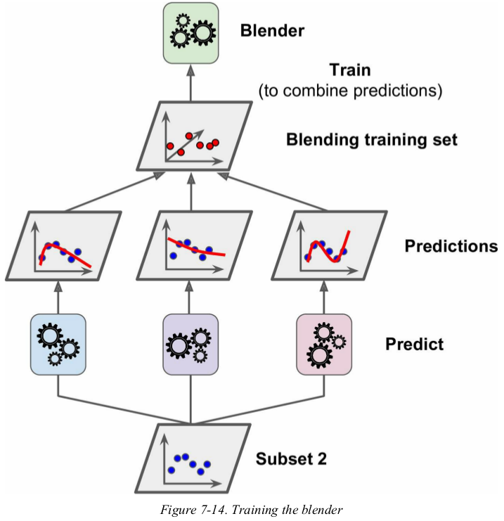
　　Figure 7-12 shows such an ensemble performing a regression task on a new instance. each of the bottom three predictors predicts a different value (3.1，2.7，and 2.9)，and then the final predictor (called a blender，or a meta learner) takes these predictions as inputs and makes the final prediction (3.0). 

　　

　　To train the blender, a common approach is to use a hold-out set.

　　First, the training set is split in two subsets. The first subset is used to train the predictors in the first layer (see Figure 7-13). 

　　

　　Next, the first layer predictors are used to make predictions on the second (held-out) set. This ensures that the predictions are “clean” . Now for each instance in the hold-out set there are three predicted values. We can create a new training set using these predicted values as input features (which makes this new training set three-dimensional), and keeping the target values. The blender is trained on this new training set, so it learns to predict the target value given the first layer’s predictions (see Figure 7-14). 没提到blender 怎么测试。

　　

　　It is actually possible to train several different blenders this way (e.g., one using Linear Regression, another using Random Forest Regression, and so on): we get a whole layer of blenders. The trick is to split the training set into three subsets: the first one is used to train the first layer, the second one is used to create the training set used to train the second layer (using predictions made by the predictors of the first layer), and the third one is used to create the training set to train the third layer (using predictions made by thepredictors of the second layer). Once this is done, we can make a prediction for a new instance by going through each layer sequentially, as shown in Figure 7-15.  有多少层就把数据集分割为几部分。

　　

　　unfortunately，Scikit-Learn doesn't support stacking directly，but it is not too hard to roll out your own implementation. 

Exercises: 

1. If you have trained five different models on the exact same training data, and they all achieve 95% precision, is there any chance that you can combine these models to get better results? If so, how? If
not, why? 

　　combine them into a voting ensemble. 

2. What is the difference between hard and soft voting classifiers?

　　a hard voting classifier just counts the votes of each classifier in the ensemble and picks the class that gets the most votes. a soft voting classifier computes the average estimated class probability for each class and picks the class with the highest probability. this gives high-confidence votes more weight and often performs better. 

3. Is it possible to speed up training of a bagging ensemble by distributing it across multiple servers? What about pasting ensembles, boosting ensembles, random forests, or stacking ensembles? 

　　regarding stacking ensembles，all the predictors in a given layer are independent of each other，so they can be trained in parallel on multiple servers. however，the predictors in one layer can only be trained after the predictors in the previous layer have all been trained. 

5. What makes Extra-Trees more random than regular Random Forests? How can this extra randomness help? Are Extra-Trees slower or faster than regular Random Forests? 

　　Extra-Trees uses random thresholds for each feature，this extra randomness acts like a form of regularization: if a Random Forest overfits the training data，Extra-Trees might perform better. 

6. If your AdaBoost ensemble underfits the training data, what hyperparameters should you tweak and how? 

　　you can try increasing the number of estimators or reducing the regularization hyperparameters of the base estimator. you may also try slightly increasing the leaning rate. 

7. If your Gradient Boosting ensemble overfits the training set, should you increase or decrease the learning rate? 

　　you should try decreasing the learning rate，you should also use early stopping to find the right number of predictors. 

8. Load the MNIST data, and split it into a training set, a validation set, and a test set. Then train various classifiers, such as a Random Forest classifier, an Extra-Trees classifier, and an SVM. Next, try to combine them into an ensemble that outperforms them all on the validation set, using a soft or hard voting classifier. Once you have found one, try it on the test set. How much better does it perform compared to the individual classifiers? 

import numpy as np
from sklearn.datasets import fetch_openml
from sklearn.model_selection import train_test_split
from sklearn.ensemble import RandomForestClassifier, ExtraTreesClassifier
from sklearn.svm import LinearSVC
from sklearn.neural_network import MLPClassifier
from sklearn.ensemble import VotingClassifier

mnist = fetch_openml('mnist_784', version=1)
mnist.target = mnist.target.astype(np.float64)

X_train_val, X_test, y_train_val, y_test = train_test_split(mnist['data'], mnist['target'], test_size=10000)
X_train, X_val, y_train, y_val = train_test_split(X_train_val, y_train_val, test_size=10000)

random_forest_clf = RandomForestClassifier(n_estimators=10, random_state=42)
extra_tree_clf = ExtraTreesClassifier(n_estimators=10, random_state=42)
svm_clf = LinearSVC(random_state=42)
mlp_clf = MLPClassifier(random_state=42)

estimators = [random_forest_clf, extra_tree_clf, svm_clf, mlp_clf]
for estimator in estimators:
    estimator.fit(X_train, y_train)

print([estimator.score(X_val, y_val) for estimator in estimators])
# [0.9434, 0.9467, 0.8568, 0.961]

named_estimators = [
    ('random_forest_clf', random_forest_clf),
    ('extra_trees_clf', extra_tree_clf),
    ('svm_clf', svm_clf),
    ('mlp_clf', mlp_clf),
]
voting_clf = VotingClassifier(named_estimators)
voting_clf.fit(X_train, y_train)
print(voting_clf.score(X_val, y_val))  # 0.9591

print([estimator.score(X_val, y_val) for estimator in voting_clf.estimators_])
# [0.9434, 0.9467, 0.8568, 0.961]  # 与上边的结果完全一样

voting_clf.set_params(svm_clf=None)  # 删除svc模型
print(voting_clf.estimators)
print(voting_clf.estimators_)

del voting_clf.estimators_[2]  # set_params不能删除已训练模型

print(voting_clf.score(X_val, y_val))  # 0.9637

# 使用soft vating
voting_clf.voting = 'soft'  # 注意：不需要重新训练
print(voting_clf.score(X_val, y_val))  # 0.9669  按理说会有显著提升

print(voting_clf.score(X_test, y_test))  # 0.9677
print([estimator.score(X_test, y_test) for estimator in voting_clf.estimators_])
# [0.9461, 0.9482, 0.9595]

9. Run the individual classifiers from the previous exercise to make predictions on the validation set, and create a new training set with the resulting predictions: each training instance is a vector containing the set of predictions from all your classifiers for an image, and the target is the image’s class. then, train a blender, and together with the classifiers they form a stacking ensemble! Now let’s evaluate the ensemble on the test set. For each image in the test set, make predictions with all your classifiers, then feed the predictions to the blender to get the ensemble’s predictions. How does it compare to the voting classifier you trained earlier? 

import numpy as np
from sklearn.datasets import fetch_openml
from sklearn.model_selection import train_test_split
from sklearn.ensemble import RandomForestClassifier, ExtraTreesClassifier
from sklearn.neural_network import MLPClassifier
from sklearn.metrics import accuracy_score

mnist = fetch_openml('mnist_784', version=1)
mnist.target = mnist.target.astype(np.float64)

X_train_val, X_test, y_train_val, y_test = train_test_split(mnist['data'], mnist['target'], test_size=10000)
X_train, X_val, y_train, y_val = train_test_split(X_train_val, y_train_val, test_size=10000)

random_forest_clf = RandomForestClassifier(n_estimators=10, random_state=42)
extra_tree_clf = ExtraTreesClassifier(n_estimators=10, random_state=42)
mlp_clf = MLPClassifier(random_state=42)

estimators = [random_forest_clf, extra_tree_clf, mlp_clf]
for estimator in estimators:
    estimator.fit(X_train, y_train)

X_val_predictions = np.empty((len(X_val), len(estimators)), dtype=np.float32)
for index, estimator in enumerate(estimators):
    X_val_predictions[:, index] = estimator.predict(X_val)

rnd_forest_blender = RandomForestClassifier(n_estimators=20, oob_score=True, random_state=42)
rnd_forest_blender.fit(X_val_predictions, y_val)

print(rnd_forest_blender.oob_score_)  # 0.9563

X_test_predictions = np.empty((len(X_test), len(estimators)), dtype=np.float32)
for index, estimator in enumerate(estimators):
    X_test_predictions[:, index] = estimator.predict(X_test)

y_pred = rnd_forest_blender.predict(X_test_predictions)
print(accuracy_score(y_test, y_pred))  # 0.9605