sklearn之聚类评估指标---轮廓系数

'''
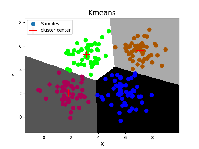
    轮廓系数：-----聚类的评估指标
            好的聚类：内密外疏，同一个聚类内部的样本要足够密集，不同聚类之间样本要足够疏远。

            轮廓系数计算规则：针对样本空间中的一个特定样本，计算它与所在聚类其它样本的平均距离a，
            以及该样本与距离最近的另一个聚类中所有样本的平均距离b，该样本的轮廓系数为(b-a)/max(a, b)，
            将整个样本空间中所有样本的轮廓系数取算数平均值，作为聚类划分的性能指标s。

            轮廓系数的区间为：[-1, 1]。 -1代表分类效果差，1代表分类效果好。0代表聚类重叠，没有很好的划分聚类。

            轮廓系数相关API：
                import sklearn.metrics as sm
                # v：平均轮廓系数
                # metric：距离算法：使用欧几里得距离(euclidean)
                v = sm.silhouette_score(输入集, 输出集, sample_size=样本数, metric=距离算法)

    案例：输出KMeans算法聚类划分后的轮廓系数。
'''

import numpy as np
import matplotlib.pyplot as mp
import sklearn.cluster as sc
import sklearn.metrics as sm

# 读取数据，绘制图像
x = np.loadtxt('./ml_data/multiple3.txt', unpack=False, dtype='f8', delimiter=',')
print(x.shape)

# 基于Kmeans完成聚类
model = sc.KMeans(n_clusters=4)
model.fit(x)  # 完成聚类
pred_y = model.predict(x)  # 预测点在哪个聚类中
print(pred_y)  # 输出每个样本的聚类标签
# 打印轮廓系数
print(sm.silhouette_score(x, pred_y, sample_size=len(x), metric='euclidean'))
# 获取聚类中心
centers = model.cluster_centers_
print(centers)

# 绘制分类边界线
l, r = x[:, 0].min() - 1, x[:, 0].max() + 1
b, t = x[:, 1].min() - 1, x[:, 1].max() + 1
n = 500
grid_x, grid_y = np.meshgrid(np.linspace(l, r, n), np.linspace(b, t, n))
bg_x = np.column_stack((grid_x.ravel(), grid_y.ravel()))
bg_y = model.predict(bg_x)
grid_z = bg_y.reshape(grid_x.shape)

# 画图显示样本数据
mp.figure('Kmeans', facecolor='lightgray')
mp.title('Kmeans', fontsize=16)
mp.xlabel('X', fontsize=14)
mp.ylabel('Y', fontsize=14)
mp.tick_params(labelsize=10)
mp.pcolormesh(grid_x, grid_y, grid_z, cmap='gray')
mp.scatter(x[:, 0], x[:, 1], s=80, c=pred_y, cmap='brg', label='Samples')
mp.scatter(centers[:, 0], centers[:, 1], s=300, color='red', marker='+', label='cluster center')
mp.legend()
mp.show()


输出结果：
(200, 2)
[1 1 0 2 1 3 0 2 1 3 0 2 1 3 0 2 1 3 0 2 1 3 0 2 3 3 0 2 1 3 0 2 1 3 0 2 1
 3 0 2 1 3 0 2 1 3 0 2 1 3 0 2 1 3 0 2 1 3 0 2 1 3 0 2 1 3 0 2 1 3 0 2 1 3
 0 2 1 3 0 2 1 3 0 2 1 3 0 2 1 3 0 2 1 3 0 2 0 3 0 2 1 3 0 2 1 3 0 2 1 3 0
 2 1 3 0 2 1 3 0 2 1 3 0 2 1 3 0 2 1 3 0 2 1 3 0 2 1 3 0 2 1 3 0 2 1 3 0 2
 1 1 0 2 1 3 0 2 1 3 0 3 1 3 0 2 1 3 0 2 1 3 0 2 1 3 0 2 1 3 0 2 1 3 0 2 1
 3 0 2 1 3 0 2 1 3 0 2 1 3 0 2]
0.5773232071896659
[[5.91196078 2.04980392]
 [1.831      1.9998    ]
 [7.07326531 5.61061224]
 [3.1428     5.2616    ]]