A geometric interpretation of the covariance matrix
Contents [hide]
Introduction
In this article, we provide an intuitive, geometric interpretation of the covariance matrix, by exploring the relation between linear transformations and the resulting data covariance. Most textbooks explain the shape of data based on the concept of covariance matrices. Instead, we take a backwards approach and explain the concept of covariance matrices based on the shape of data.
In a previous article, we discussed the concept of variance, and provided a derivation and proof of the well known formula to estimate the sample variance. Figure 1 was used in this article to show that the standard deviation, as the square root of the variance, provides a measure of how much the data is spread across the feature space.

Figure 1. Gaussian density function. For normally distributed data, 68% of the samples fall within the interval defined by the mean plus and minus the standard deviation.
We showed that an unbiased estimator of the sample variance can be obtained by:
(1) 
However, variance can only be used to explain the spread of the data in the directions parallel to the axes of the feature space. Consider the 2D feature space shown by figure 2:

Figure 2. The diagnoal spread of the data is captured by the covariance.
For this data, we could calculate the variance  in the x-direction and the variance
  in the y-direction. However, the horizontal spread and the vertical spread of the data does not explain the clear diagonal correlation. Figure 2 clearly shows that on average, if the x-value of a data point increases, then also the y-value increases, resulting in a positive correlation. This correlation can be captured by extending the notion of variance to what is called the ‘covariance’ of the data:
(2) 
For 2D data, we thus obtain , ,  and
and  . These four values can be summarized in a matrix, called the covariance matrix:
(3) 
If x is positively correlated with y, y is also positively correlated with x. In other words, we can state that  . Therefore, the covariance matrix is always a symmetric matrix with the variances on its diagonal and the covariances off-diagonal. Two-dimensional normally distributed data is explained completely by its mean and its
  covariance matrix. Similarly, a
  covariance matrix is used to capture the spread of three-dimensional data, and a
  covariance matrix captures the spread of N-dimensional data.
Figure 3 illustrates how the overall shape of the data defines the covariance matrix:

Figure 3. The covariance matrix defines the shape of the data. Diagonal spread is captured by the covariance, while axis-aligned spread is captured by the variance.
Eigendecomposition of a covariance matrix
In the next section, we will discuss how the covariance matrix can be interpreted as a linear operator that transforms white data into the data we observed. However, before diving into the technical details, it is important to gain an intuitive understanding of how eigenvectors and eigenvalues uniquely define the covariance matrix, and therefore the shape of our data.
As we saw in figure 3, the covariance matrix defines both the spread (variance), and the orientation (covariance) of our data. So, if we would like to represent the covariance matrix with a vector and its magnitude, we should simply try to find the vector that points into the direction of the largest spread of the data, and whose magnitude equals the spread (variance) in this direction.
If we define this vector as  , then the projection of our data
  onto this vector is obtained as
  , and the variance of the projected data is
  . Since we are looking for the vector that points into the direction of the largest variance, we should choose its components such that the covariance matrix of the projected data is as large as possible. Maximizing any function of the form with respect to , where is a normalized unit vector, can be formulated as a so called Rayleigh Quotient. The maximum of such a Rayleigh Quotient is obtained by setting equal to the largest eigenvector of matrix
  .
.
In other words, the largest eigenvector of the covariance matrix always points into the direction of the largest variance of the data, and the magnitude of this vector equals the corresponding eigenvalue. The second largest eigenvector is always orthogonal to the largest eigenvector, and points into the direction of the second largest spread of the data.
Now let’s have a look at some examples. In an earlier article we saw that a linear transformation matrix  is completely defined by itseigenvectors and eigenvalues. Applied to the covariance matrix, this means that:
(4) 
where is an eigenvector of , and  is the corresponding eigenvalue.
If the covariance matrix of our data is a diagonal matrix, such that the covariances are zero, then this means that the variances must be equal to the eigenvalues . This is illustrated by figure 4, where the eigenvectors are shown in green and magenta, and where the eigenvalues clearly equal the variance components of the covariance matrix.
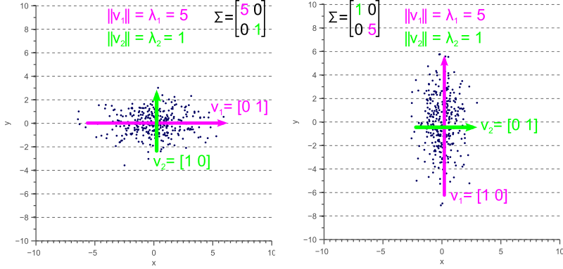
Figure 4. Eigenvectors of a covariance matrix
However, if the covariance matrix is not diagonal, such that the covariances are not zero, then the situation is a little more complicated. The eigenvalues still represent the variance magnitude in the direction of the largest spread of the data, and the variance components of the covariance matrix still represent the variance magnitude in the direction of the x-axis and y-axis. But since the data is not axis aligned, these values are not the same anymore as shown by figure 5.
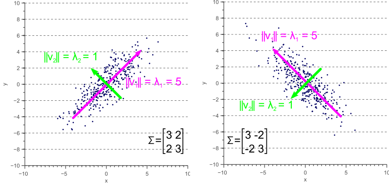
Figure 5. Eigenvalues versus variance
By comparing figure 5 with figure 4, it becomes clear that the eigenvalues represent the variance of the data along the eigenvector directions, whereas the variance components of the covariance matrix represent the spread along the axes. If there are no covariances, then both values are equal.
Covariance matrix as a linear transformation
Now let’s forget about covariance matrices for a moment. Each of the examples in figure 3 can simply be considered to be a linearly transformed instance of figure 6:

Figure 6. Data with unit covariance matrix is called white data.
Let the data shown by figure 6 be , then each of the examples shown by figure 3 can be obtained by linearly transforming :
(5) 
where is a transformation matrix consisting of a rotation matrix  and a scaling matrix
  :
:
(6) 
These matrices are defined as:
(7) 
where  is the rotation angle, and:
(8) 
where  and
and  are the scaling factors in the x direction and the y direction respectively.
In the following paragraphs, we will discuss the relation between the covariance matrix , and the linear transformation matrix  .
.
Let’s start with unscaled (scale equals 1) and unrotated data. In statistics this is often refered to as ‘white data’ because its samples are drawn from a standard normal distribution and therefore correspond to white (uncorrelated) noise:
Figure 7. White data is data with a unit covariance matrix.
The covariance matrix of this ‘white’ data equals the identity matrix, such that the variances and standard deviations equal 1 and the covariance equals zero:
(9) 
Now let’s scale the data in the x-direction with a factor 4:
(10) 
The data  now looks as follows:

Figure 8. Variance in the x-direction results in a horizontal scaling.
The covariance matrix  of is now:
(11) 
Thus, the covariance matrix of the resulting data is related to the linear transformation that is applied to the original data as follows:  , where
(12) 
However, although equation (12) holds when the data is scaled in the x and y direction, the question rises if it also holds when a rotation is applied. To investigate the relation between the linear transformation matrix and the covariance matrix in the general case, we will therefore try to decompose the covariance matrix into the product of rotation and scaling matrices.
As we saw earlier, we can represent the covariance matrix by its eigenvectors and eigenvalues:
(13)
where is an eigenvector of , and is the corresponding eigenvalue.
Equation (13) holds for each eigenvector-eigenvalue pair of matrix . In the 2D case, we obtain two eigenvectors and two eigenvalues. The system of two equations defined by equation (13) can be represented efficiently using matrix notation:
(14) 
where  is the matrix whose columns are the eigenvectors of and
  is the diagonal matrix whose non-zero elements are the corresponding eigenvalues.
This means that we can represent the covariance matrix as a function of its eigenvectors and eigenvalues:
(15) 
Equation (15) is called the eigendecomposition of the covariance matrix and can be obtained using a Singular Value Decompositionalgorithm. Whereas the eigenvectors represent the directions of the largest variance of the data, the eigenvalues represent the magnitude of this variance in those directions. In other words, represents a rotation matrix, while  represents a scaling matrix. The covariance matrix can thus be decomposed further as:
(16) 
where  is a rotation matrix and
  is a scaling matrix.
In equation (6) we defined a linear transformation  . Since is a diagonal scaling matrix,
  . Furthermore, since is an orthogonal matrix,
  . Therefore,
  . The covariance matrix can thus be written as:
(17) 
In other words, if we apply the linear transformation defined by to the original white data shown by figure 7, we obtain the rotated and scaled data with covariance matrix  . This is illustrated by figure 10:

Figure 10. The covariance matrix represents a linear transformation of the original data.
The colored arrows in figure 10 represent the eigenvectors. The largest eigenvector, i.e. the eigenvector with the largest corresponding eigenvalue, always points in the direction of the largest variance of the data and thereby defines its orientation. Subsequent eigenvectors are always orthogonal to the largest eigenvector due to the orthogonality of rotation matrices.
Conclusion
In this article we showed that the covariance matrix of observed data is directly related to a linear transformation of white, uncorrelated data. This linear transformation is completely defined by the eigenvectors and eigenvalues of the data. While the eigenvectors represent the rotation matrix, the eigenvalues correspond to the square of the scaling factor in each dimension.
If you’re new to this blog, don’t forget to subscribe, or follow me on twitter!