python回归分析

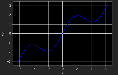
假设原函数由一个三角函数和一个线性项组成

import numpy as np
import matplotlib.pyplot as plt
%matplotlib inline

def f(x):
    return np.sin(x) + 0.5 * x

x = np.linspace(-2 * np.pi, 2 * np.pi, 50)

plt.plot(x, f(x), 'b')
plt.grid(True)
plt.xlabel('x')
plt.ylabel('f(x)')

一、用回归方式逼近

1. 作为基函数的单项式

最简单的情况是以单项式为基函数——也就是说，b₁=1,b₂=x,b₃=x²,b₄=x³,... 在这种情况下，Numpy有确定最优参数（polyfit）和以一组输入值求取近似值（ployval）的内建函数。ployfit函数参数如下：

参数	描述
x	x坐标（自变量值）
y	y坐标（因变量值）
deg	多项式拟合度
full	如果有真，返回额外的诊断信息
w	应用到y坐标的权重
cov	如果为真，返回协方差矩阵

典型向量化风格的polyfit和polyval线性回归（deg=7）应用方式如下：

reg = np.polyfit(x, f(x), deg=7)
ry = np.polyval(reg, x)
plt.plot(x,f(x),'b',label='f(x)')
plt.plot(x,ry,'r.',label='regression')
plt.grid(True)
plt.xlabel('x')
plt.ylabel('f(x)')

 

2. 单独的基函数

当选择更好的基函数组时，可以得到更好的回归结果。单独的基函数必须能通过一个矩阵方法定义（使用Numpy ndarray对象）。

numpy.linalg子库提供lstsq函数，以解决最小二乘化做问题

matrix = np.zeros((3+1,len(x)))
matrix[3,:] = np.sin(x)
matrix[2,:] = x **2
matrix[1,:] = x
matrix[0,:] = 1

reg = np.linalg.lstsq(matrix.T,f(x))[0]
ry = np.dot(reg,matrix)

plt.plot(x,f(x),'b',label='f(x)')
plt.plot(x,ry,'r.',label='regression')
plt.legend(loc = 0)
plt.grid(True)
plt.xlabel('x')
plt.ylabel('f(x)')

 对于有噪声的数据，未排序的数据，回归法都可处理。

3. 多维

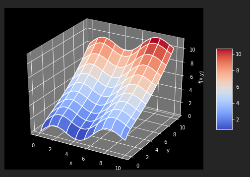
以fm函数为例

def fm(x,y):
    return np.sin(x) + 0.25 *x +np.sqrt(y) + 0.05 * y **2

x = np.linspace(0,10,20)
y = np.linspace(0,10,20)
X, Y = np.meshgrid(x,y)
Z = fm(X,Y)
x = X.flatten()
y = Y.flatten()

from mpl_toolkits.mplot3d import Axes3D
import matplotlib as mpl

fig = plt.figure(figsize=(9, 6))
ax = fig.gca(projection='3d')
surf = ax.plot_surface(X,Y,Z,rstride=2,cstride=2,cmap=mpl.cm.coolwarm,linewidth=0.5,antialiased=True)
ax.set_xlabel('x')
ax.set_ylabel('y')
ax.set_zlabel('f(x,y)')
fig.colorbar(surf,shrink=0.5,aspect=5)

为了获得好的回归结果，编译一组基函数，包括一个sin函数和sqrt函数。statsmodels库提供相当通过和有益的函数OLS，可以用于一维和多维最小二乘回归。

matrix = np.zeros((len(x),6+1))
matrix[:,6] = np.sqrt(y)
matrix[:,5] = np.sin(x)
matrix[:,4] = y ** 2
matrix[:,3] = x **2 
matrix[:,2] = y
matrix[:,1] = x
matrix[:,0] = 1

import statsmodels.api as sm 
model = sm.OLS(fm(x,y),matrix).fit()

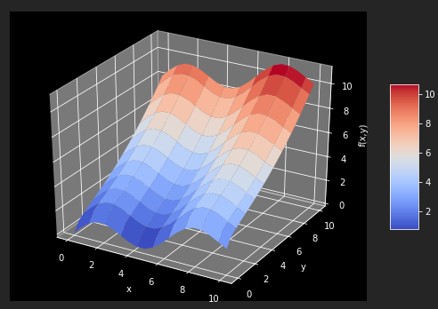
OSL函数的好处之一是提供关于回归及其而非结果的大量几百万来看信息。调用model.summary可以访问结果的一个摘要。单独统计数字（如确定系数）通常可以直接访问model.rsquared。最优回归系数，保存在model对象的params属性中。

model.rsquared
a = model.params

def reg_func(a,x,y):
    f6 = a[6] * np.sqrt(y)
    f5 = a[5] * np.sin(x)
    f4 = a[4] * y ** 2
    f3 = a[3] * x ** 2
    f2 = a[2] * y
    f1 = a[1] * x
    f0 = a[0] * 1
    return (f6+f5+f4+f3+f2+f1+f0)
# reg_func返回给定最优回归参数和自变量数据点的回归函数值
RZ = reg_func(a,X,Y)
fig = plt.figure(figsize=(9, 6))
ax = fig.gca(projection='3d')
surf1 = ax.plot_surface(X,Y,Z,rstride=2,cstride=2,cmap=mpl.cm.coolwarm,linewidth=0.5,antialiased=True)
surf2 = ax.plot_wireframe(X,Y,RZ,rstride=2,cstride=2,label = 'regression')
ax.set_xlabel('x')
ax.set_ylabel('y')
ax.set_zlabel('f(x,y)')
fig.colorbar(surf,shrink=0.5,aspect=5)