【12月DW打卡】joyful-pandas

第十章 时序数据

小结

• 原文链接: https://datawhalechina.github.io/joyful-pandas/build/html/目录/ch10.html
• Offset aliases的freq链接速查: https://pandas.pydata.org/docs/user_guide/timeseries.html#offset-aliases
• resample源文档: https://pandas.pydata.org/docs/user_guide/timeseries.html#resampling
  其他
• 转换命令 jupyter nbconvert --to markdown E:PycharmProjectsTianChiProject0_山枫叶纷飞competitions08_joyful-pandas10_pandas时序数据.ipynb

import numpy as np
import pandas as pd
file_prefix = 'E:\PycharmProjects\DatawhaleChina\joyful-pandas\data\'
print(file_prefix)

E:PycharmProjectsDatawhaleChinajoyful-pandasdata

一、时序中的基本对象

总结出官方文档中的这个表格：

• datetime64[ns] 本质上可以理解为一个大整数，对于一个该类型的序列，可以使用 max, min, mean ，来取得最大时间戳、最小时间戳和“平均”时间戳。

概念	单元素类型	数组类型	pandas数据类型
Date times	Timestamp	DatetimeIndex	datetime64[ns]
Time deltas(时间差)	Timedelta	TimedeltaIndex	timedelta64[ns]
Time spans	Period	PeriodIndex	period[freq]
Date offsets	DateOffset	None	None

二、时间戳

1. Timestamp的构造与属性

单个时间戳的生成利用 pd.Timestamp 实现，一般而言的常见日期格式都能被成功地转换

ts = pd.Timestamp('2020/1/1')
ts

Timestamp('2020-01-01 00:00:00')

通过year, month, day, hour, min, second可以获取具体的数值：

ts.year

2020

在pandas中，时间戳的最小精度为纳秒ns，由于使用了64位存储，可以表示的时间范围大约可以如下计算：

[ m Time\,Range = frac{2^{64}}{10^9 imes 60 imes 60 imes 24 imes 365} approx 585 (Years) ]

通过pd.Timestamp.max和pd.Timestamp.min可以获取时间戳表示的范围，可以看到确实表示的区间年数大小正如上述计算结果：

print(pd.Timestamp.max)
print(pd.Timestamp.min)

2262-04-11 23:47:16.854775807
1677-09-21 00:12:43.145225

pd.Timestamp.max.year - pd.Timestamp.min.year

585

2. Datetime序列的生成

一组时间戳可以组成时间序列，可以用to_datetime和date_range来生成。其中，to_datetime能够把一列时间戳格式的对象转换成为datetime64[ns]类型的时间序列：

# 生存DatetimeIndex类型
pd.to_datetime(['2020-1-1', '2020-1-3', '2020-1-6'])

DatetimeIndex(['2020-01-01', '2020-01-03', '2020-01-06'], dtype='datetime64[ns]', freq=None)

时间戳的格式不满足转换时，可以强制使用 format 进行匹配：

temp = pd.to_datetime(['2020\1\1','2020\1\3'],format='%Y\%m\%d')
temp

DatetimeIndex(['2020-01-01', '2020-01-03'], dtype='datetime64[ns]', freq=None)

# 显式用 Series 转化,转为 datetime64[ns] 的序列
temp = pd.to_datetime(pd.Series(['2020\1\1','2020\1\3']), format='%Y\%m\%d')
temp

0   2020-01-01
1   2020-01-03
dtype: datetime64[ns]

另外，还存在一种把表的多列时间属性拼接转为时间序列的 to_datetime 操作，此时的列名必须和以下给定的时间关键词列名一致：

df_date_cols = pd.DataFrame({'year': [2020, 2020],
                             'month': [1, 1],
                             'day': [1, 2],
                             'hour': [10, 20],
                             'minute': [30, 50],
                             'second': [20, 40]})
pd.to_datetime(df_date_cols)

0   2020-01-01 10:30:20
1   2020-01-02 20:50:40
dtype: datetime64[ns]

date_range是一种生成连续间隔时间的一种方法，其重要的参数为start, end, freq, periods，它们分别表示开始时间，结束时间，时间间隔，时间戳个数。其中，四个中的三个参数决定了，那么剩下的一个就随之确定了。这里要注意，开始或结束日期如果作为端点则它会被包含：

pd.date_range('2020-1-1','2020-1-21', freq='10D') # 包含

DatetimeIndex(['2020-01-01', '2020-01-11', '2020-01-21'], dtype='datetime64[ns]', freq='10D')

date_range 是一种生成连续间隔时间的一种方法，
其重要的参数为
start, 开始时间
end, 结束时间
freq, 时间间隔
periods, 时间戳个数

(其中，四个中的三个参数决定了，那么剩下的一个就随之确定了。这里要注意，开始或结束日期如果作为端点则它会被包含)

3. dt对象

如同 category, string 的(Series)序列上定义了 cat, str 来完成分类数据和文本数据的操作，在时序类型的序列上定义了 dt 对象来完成许多时间序列的相关操作。

这里对于 datetime64[ns] 类型而言，可以大致分为三类操作：取出时间相关的属性、判断时间戳是否满足条件、取整操作。

3.1 取出时间相关的属

第一类操作的常用属性包括： date, time, year, month, day, hour, minute, second, microsecond, nanosecond, dayofweek, dayofyear, weekofyear, daysinmonth, quarter ，其中 daysinmonth, quarter 分别表示月中的第几天和季度。

3.2 判断时间戳是否满足条件

第二类判断操作主要用于测试是否为月/季/年的第一天或者最后一天：(可选is_year/quarter/month_start)

s = pd.Series(pd.date_range('2020-1-1','2020-1-3', freq='D'))
s.dt.is_year_start # 还可选 is_quarter/month_start

0     True
1    False
2    False
dtype: bool

3.3 取整操作

第三类的取整操作包含round, ceil, floor，它们的公共参数为freq，常用的包括H, min, S（小时、分钟、秒），所有可选的freq可参考此处。

round, ceil, floor

• round: 四舍五入
• ceil : 向上取整
• floor: 向下取整

s = pd.Series(pd.date_range('2020-1-1 20:35:00', '2020-1-1 22:35:00', freq='45min'))
s

0   2020-01-01 20:35:00
1   2020-01-01 21:20:00
2   2020-01-01 22:05:00
dtype: datetime64[ns]

s.dt.round('1H')

0   2020-01-01 21:00:00
1   2020-01-01 21:00:00
2   2020-01-01 22:00:00
dtype: datetime64[ns]

4. 时间戳的切片与索引

一般而言，时间戳序列作为索引使用。如果想要选出某个子时间戳序列，第一类方法是利用 dt 对象和布尔条件联合使用，另一种方式是利用切片，后者常用于连续时间戳。

# 是利用 dt 对象和布尔条件联合使用
s = pd.Series(np.random.randint(2,size=366), index=pd.date_range('2020-01-01','2020-12-31'))
idx = s.index
idx

DatetimeIndex(['2020-01-01', '2020-01-02', '2020-01-03', '2020-01-04',
               '2020-01-05', '2020-01-06', '2020-01-07', '2020-01-08',
               '2020-01-09', '2020-01-10',
               ...
               '2020-12-22', '2020-12-23', '2020-12-24', '2020-12-25',
               '2020-12-26', '2020-12-27', '2020-12-28', '2020-12-29',
               '2020-12-30', '2020-12-31'],
              dtype='datetime64[ns]', length=366, freq='D')

print('dt对象和布尔条件联合, 求得每月的第一天或者最后一天')
idx = pd.Series(idx)
s[(idx.dt.is_month_start|idx.dt.is_month_end).values].head()

dt对象和布尔条件联合, 求得每月的第一天或者最后一天





2020-01-01    0
2020-01-31    0
2020-02-01    1
2020-02-29    1
2020-03-01    1
dtype: int32

Example2：计算双休日

print(idx.dt.dayofweek.isin([5,6]).values[0:5], '....')
s[idx.dt.dayofweek.isin([5,6]).values].head()

[False False False  True  True] ....





2020-01-04    1
2020-01-05    1
2020-01-11    0
2020-01-12    0
2020-01-18    0
dtype: int32

Example5：取出5月初至7月15日

s['2020-05':'2020-7-15'].head()

2020-05-01    1
2020-05-02    0
2020-05-03    0
2020-05-04    1
2020-05-05    0
Freq: D, dtype: int32

s[(s.index>='2020-05')&(s.index<='2020-7-15')].head()

2020-05-01    1
2020-05-02    0
2020-05-03    0
2020-05-04    1
2020-05-05    0
Freq: D, dtype: int32

三、时间差

1. Timedelta的生成

时间差可以理解为两个时间戳的差，这里也可以通过pd.Timedelta来构造：

pd.Timestamp('20200102 08:00:00') - pd.Timestamp('20200101 07:35:00')

Timedelta('1 days 00:25:00')

pd.Timedelta(days=1, minutes=25) # 需要注意加s

Timedelta('1 days 00:25:00')

生成时间差序列的主要方式是 pd.to_timedelta ，其类型为 timedelta64[ns];
与 date_range 一样，时间差序列也可以用 timedelta_range 来生成，它们两者具有一致的参数：

pd.timedelta_range('0s', '1000s', freq='6min')

TimedeltaIndex(['0 days 00:00:00', '0 days 00:06:00', '0 days 00:12:00'], dtype='timedelta64[ns]', freq='6T')

pd.timedelta_range('0s', '1000s', periods=3)

TimedeltaIndex(['0 days 00:00:00', '0 days 00:08:20', '0 days 00:16:40'], dtype='timedelta64[ns]', freq=None)

对于 Timedelta 序列，同样也定义了 dt 对象，上面主要定义了的属性包括 days, seconds, mircroseconds, nanoseconds ，它们分别返回了对应的时间差特征。需要注意的是，这里的 seconds 不是指单纯的秒，而是对天数取余后剩余的秒数[将 days, seconds, mircroseconds, nanoseconds 的结果进行汇总可以得到原值]：

t_delta = pd.Series(pd.timedelta_range('0s', '1000s', periods=3))
t_delta.dt.seconds.head()

0       0
1     500
2    1000
dtype: int64

与时间戳序列类似，取整函数也是可以在 dt 对象上使用的：

t_delta.dt.round('min').head()

0   0 days 00:00:00
1   0 days 00:08:00
2   0 days 00:17:00
dtype: timedelta64[ns]

2. Timedelta的运算
   时间差支持的常用运算有三类：与标量的乘法运算、与时间戳的加减法运算、与时间差的加减法与除法运算：

td1 = pd.Timedelta(days=1)
td2 = pd.Timedelta(days=3)
ts = pd.Timestamp('20200101')

print('与标量的乘法运算, 仅支持乘法')
td1*2

与标量的乘法运算, 仅支持乘法





Timedelta('2 days 00:00:00')

print('与时间戳的加减法运算')
ts+td1

与时间戳的加减法运算





Timestamp('2020-01-02 00:00:00')

print('与时间差的加减法与除法运算')
td1 + ts # 逐个相加

与时间差的加减法与除法运算





Timestamp('2020-01-02 00:00:00')

四、日期偏置

1. 简介

日期偏置是一种和日历相关的特殊时间差，例如回到第一节中的两个问题：如何求2020年9月第一个周一的日期，以及如何求2020年9月7日后的第30个工作日是哪一天。
Offset 对象在 pd.offsets 中被定义。当使用 + 时获取离其最近的下一个日期，当使用 - 时获取离其最近的上一个日期：

pd.Timestamp('20200831') - pd.offsets.WeekOfMonth(week=0,weekday=0)

Timestamp('2020-08-03 00:00:00')

pd.Timestamp('20200907') - pd.offsets.BDay(30)

Timestamp('2020-07-27 00:00:00')

pd.Timestamp('20200907') + pd.offsets.MonthEnd()

Timestamp('2020-09-30 00:00:00')

常用的日期偏置如下可以查阅这里的文档描述。在文档罗列的Offset中，需要介绍一个特殊的Offset对象CDay，其中的holidays, weekmask参数能够分别对自定义的日期和星期进行过滤，前者传入了需要过滤的日期列表，后者传入的是三个字母的星期缩写构成的星期字符串，其作用是只保留字符串中出现的星期：

my_filter = pd.offsets.CDay(n=1,weekmask='Wed Fri',holidays=['20200109'])
dr = pd.date_range('2020-01-08', '2020-01-11')
dr.to_series().dt.dayofweek

2020-01-08    2
2020-01-09    3
2020-01-10    4
2020-01-11    5
Freq: D, dtype: int64

print('开启过滤')
[i + my_filter for i in dr]

开启过滤





[Timestamp('2020-01-10 00:00:00'),
 Timestamp('2020-01-10 00:00:00'),
 Timestamp('2020-01-15 00:00:00'),
 Timestamp('2020-01-15 00:00:00')]

print('`1-n`表示增加一天`CDay`，`dr`中的第一天为`20200108`，但由于下一天`20200109`被排除了，并且`20200110`是合法的周五，因此转为`20200110`，其他后面的日期处理类似。')

`1-n`表示增加一天`CDay`，`dr`中的第一天为`20200108`，但由于下一天`20200109`被排除了，并且`20200110`是合法的周五，因此转为`20200110`，其他后面的日期处理类似。

【CAUTION】不要使用部分Offset

在当前版本下由于一些 bug ，不要使用 Day 级别以下的 Offset 对象，比如 Hour, Second 等，请使用对应的 Timedelta 对象来代替。

2. 偏置字符串（freq）

前面提到了关于date_range的freq取值可用Offset对象，同时在pandas中几乎每一个Offset对象绑定了日期偏置字符串（frequencies strings/offset aliases），可以指定Offset对应的字符串来替代使用。下面举一些常见的例子。

pd.date_range('20200101','20200110', freq='B') # 工作日

DatetimeIndex(['2020-01-01', '2020-01-02', '2020-01-03', '2020-01-06',
               '2020-01-07', '2020-01-08', '2020-01-09', '2020-01-10'],
              dtype='datetime64[ns]', freq='B')

pd.date_range('20200101','20200201', freq='W-MON') # 周一

DatetimeIndex(['2020-01-06', '2020-01-13', '2020-01-20', '2020-01-27'], dtype='datetime64[ns]', freq='W-MON')

上面的这些字符串，等价于使用如下的 Offset 对象：

pd.date_range('20200101','20200110', freq=pd.offsets.BDay()) # 工作日

DatetimeIndex(['2020-01-01', '2020-01-02', '2020-01-03', '2020-01-06',
               '2020-01-07', '2020-01-08', '2020-01-09', '2020-01-10'],
              dtype='datetime64[ns]', freq='B')

pd.date_range('20200101','20200201', freq=pd.offsets.WeekOfMonth(week=0, weekday=0)) # 周一

DatetimeIndex(['2020-01-06'], dtype='datetime64[ns]', freq='WOM-1MON')

3. 滑动窗口

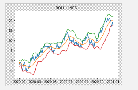
所谓时序的滑窗函数，即把滑动窗口用freq关键词代替，下面给出一个具体的应用案例：在股票市场中有一个指标为BOLL指标，它由中轨线、上轨线、下轨线这三根线构成，具体的计算方法分别是N日均值线、N日均值加两倍N日标准差线、N日均值减两倍N日标准差线。

利用rolling对象计算N=30的BOLL指标可以如下写出：

import matplotlib.pyplot as plt
idx = pd.date_range('20200101', '20201231', freq='B')
np.random.seed(2020)
data = np.random.randint(-1,2,len(idx)).cumsum() # 随机游动构造模拟序列
s = pd.Series(data,index=idx)
s.head()

2020-01-01   -1
2020-01-02   -2
2020-01-03   -1
2020-01-06   -1
2020-01-07   -2
Freq: B, dtype: int32

r = s.rolling('30D')
plt.plot(s)
plt.title('BOLL LINES')
plt.plot(r.mean())
plt.plot(r.mean()+r.std()*2)
plt.plot(r.mean()-r.std()*2)

[<matplotlib.lines.Line2D at 0x2380ee12ac8>]

对于shift函数而言，作用在datetime64为索引的序列上时，可以指定freq单位进行滑动：

s.shift(freq='50D').head()

2020-02-20   -1
2020-02-21   -2
2020-02-22   -1
2020-02-25   -1
2020-02-26   -2
dtype: int32

另外，datetime64[ns]的序列进行diff后就能够得到timedelta64[ns]的序列，这能够使用户方便地观察有序时间序列的间隔：

my_series = pd.Series(s.index)
my_series.head()
my_series.diff(1).head()

0      NaT
1   1 days
2   1 days
3   3 days
4   1 days
dtype: timedelta64[ns]

4. 重采样

重采样对象 resample 和第四章中分组对象 groupby 的用法类似，前者是针对时间序列的分组计算而设计的分组对象。

• 支持常规gp的操作
• 支持自定义的apply函数
• 坑很多,建议直接看源文档 https://pandas.pydata.org/docs/user_guide/timeseries.html#resampling

六、练习

Ex1：太阳辐射数据集

现有一份关于太阳辐射的数据集：

import numpy as np
import pandas as pd
import matplotlib.pyplot as plt
file_prefix = 'E:\PycharmProjects\DatawhaleChina\joyful-pandas\data\'

solar_df = pd.read_csv(file_prefix + 'solar.csv', usecols=['Data','Time','Radiation','Temperature'])
solar_df.head(3)

	Data	Time	Radiation	Temperature
0	9/29/2016 12:00:00 AM	23:55:26	1.21	48
1	9/29/2016 12:00:00 AM	23:50:23	1.21	48
2	9/29/2016 12:00:00 AM	23:45:26	1.23	48

1. 将Datetime, Time合并为一个时间列Datetime，同时把它作为索引后排序。

print(solar_df.head(3))

                    Data      Time  Radiation  Temperature
0  9/29/2016 12:00:00 AM  23:55:26       1.21           48
1  9/29/2016 12:00:00 AM  23:50:23       1.21           48
2  9/29/2016 12:00:00 AM  23:45:26       1.23           48

df = solar_df.copy()
df['Data'] = df['Data'].apply(lambda x: str(x).split(' ')[0])
df['Datetime'] = pd.to_datetime(df['Data'] +' '+ df['Time'])
df = df.drop(labels=['Data', 'Time'], axis=1).set_index('Datetime').sort_index()
df.head()

	Radiation	Temperature
Datetime
2016-09-01 00:00:08	2.58	51
2016-09-01 00:05:10	2.83	51
2016-09-01 00:20:06	2.16	51
2016-09-01 00:25:05	2.21	51
2016-09-01 00:30:09	2.25	51

2. 每条记录时间的间隔显然并不一致，请解决如下问题：

• 找出间隔时间的前三个最大值所对应的三组时间戳。

print('total: ',df.shape)
print('尝试生成delta: ')
timedelt = pd.to_timedelta(np.diff(df.index), errors="raise")
print('timedelt: ',timedelt.shape)
print(timedelt[0:5])

total:  (32686, 2)
尝试生成delta: 
timedelt:  (32685,)
TimedeltaIndex(['0 days 00:05:02', '0 days 00:14:56', '0 days 00:04:59',
                '0 days 00:05:04', '0 days 00:14:55'],
               dtype='timedelta64[ns]', freq=None)

delt = timedelt.to_series().reset_index(drop=True).dt.total_seconds()
max_pairs_idxs = delt.nlargest(3).index
print('max_pairs_idxs: ', max_pairs_idxs)
tuples = max_pairs_idxs.union(max_pairs_idxs-1)
df.index[tuples]

max_pairs_idxs:  Int64Index([25922, 24521, 7416], dtype='int64')





DatetimeIndex(['2016-09-29 23:50:23', '2016-09-29 23:55:26',
               '2016-11-29 19:00:03', '2016-11-29 19:05:02',
               '2016-12-05 20:41:07', '2016-12-05 20:45:53'],
              dtype='datetime64[ns]', name='Datetime', freq=None)

• 是否存在一个大致的范围，使得绝大多数的间隔时间都落在这个区间中？如果存在，请对此范围内的样本间隔秒数画出柱状图，设置bins=50。

print('排序后,使用分位数直接分为0.99')
mask_res = df.mask((df > df.quantile(0.99))|(df < df.quantile(0.01)))
mask_res.dropna(inplace=True)

排序后,使用分位数直接分为0.99

print('绘制直方图: ')
# plt.hist(mask_res, bins=50)
print('莫名卡死了~~~内存条崩了一根!')

绘制直方图: 
莫名卡死了~~~内存条崩了一根!

3. 求如下指标对应的Series：

• 温度与辐射量的6小时滑动相关系数

# Radiation	Temperature
df['Radiation'].rolling('6H').corr(df['Temperature'])

Datetime
2016-09-01 00:00:08         NaN
2016-09-01 00:05:10         NaN
2016-09-01 00:20:06         inf
2016-09-01 00:25:05        -inf
2016-09-01 00:30:09        -inf
                         ...   
2016-12-31 23:35:02    0.416187
2016-12-31 23:40:01    0.416565
2016-12-31 23:45:04    0.328574
2016-12-31 23:50:03    0.261883
2016-12-31 23:55:01    0.262406
Length: 32686, dtype: float64

• 以三点、九点、十五点、二十一点为分割，该观测所在时间区间的温度均值序列

df['Temperature'].resample('6H', origin='03:00:00').mean()

Datetime
2016-08-31 21:00:00    51.218750
2016-09-01 03:00:00    50.033333
2016-09-01 09:00:00    59.379310
2016-09-01 15:00:00    57.984375
2016-09-01 21:00:00    51.393939
                         ...    
2016-12-30 21:00:00    43.902778
2016-12-31 03:00:00    42.708333
2016-12-31 09:00:00    51.513889
2016-12-31 15:00:00    48.555556
2016-12-31 21:00:00    41.111111
Freq: 6H, Name: Temperature, Length: 489, dtype: float64

• 每个观测6小时前的辐射量（一般而言不会恰好取到，此时取最近时间戳对应的辐射量）
  参考答案: (我不知道这题意说的啥 !!!!)

In [222]: my_dt = df.index.shift(freq='-6H')

In [223]: int_loc = [df.index.get_loc(i, method='nearest') for i in my_dt]

In [224]: res = df.Radiation.iloc[int_loc]

In [225]: res.tail(3)
Out[225]:
Datetime
2016-12-31 17:45:02    9.33
2016-12-31 17:50:01    8.49
2016-12-31 17:55:02    5.84
Name: Radiation, dtype: float64

Ex2：水果销量数据集

现有一份2019年每日水果销量记录表：

fruit_df = pd.read_csv(file_prefix + 'fruit.csv')
fruit_df.head(3)

	Date	Fruit	Sale
0	2019-04-18	Peach	15
1	2019-12-29	Peach	15
2	2019-06-05	Peach	19

1. 统计如下指标：

• 每月上半月（15号及之前）与下半月葡萄销量的比值

df = fruit_df.copy()
df['Date'] = pd.to_datetime(df['Date'])
# df.set_index('Date', inplace=True)
print(set(np.array(df['Fruit'])))

# Grape
# https://pandas.pydata.org/docs/user_guide/timeseries.html#offset-aliases  对应的aliase为 SMS  SM
df_grape = df[df['Fruit']=='Grape']
df_grape.head()

{'Grape', 'Apple', 'Banana', 'Peach', 'Pear'}

	Date	Fruit	Sale
5	2019-05-19	Grape	17
12	2019-06-16	Grape	28
17	2019-08-11	Grape	25
18	2019-03-29	Grape	20
25	2019-07-09	Grape	13

df_grape.Date.dt.day<=15

5        False
12       False
17        True
18       False
25        True
         ...  
19982     True
19984    False
19985     True
19986     True
19990     True
Name: Date, Length: 4368, dtype: bool

res = df_grape.groupby([np.where(df_grape.Date.dt.day<=15,
                         'First', 'Second'),df_grape.Date.dt.month])['Sale'].mean()
res

        Date
First   1       66.349462
        2       59.447059
        3       57.502890
        4       60.437838
        5       57.135593
        6       64.923977
        7       65.653631
        8       64.651515
        9       63.297436
        10      61.514851
        11      58.608696
        12      60.252941
Second  1       56.467742
        2       61.355828
        3       60.443396
        4       59.206522
        5       61.366120
        6       55.798030
        7       55.407643
        8       62.047619
        9       59.117647
        10      61.170854
        11      57.108108
        12      61.976048
Name: Sale, dtype: float64

# droplevel 把Date下的first和second给拆分单拎出来
ret_frame = res.to_frame().unstack(0).droplevel(0,axis=1)
ret_frame

	First	Second
Date
1	66.349462	56.467742
2	59.447059	61.355828
3	57.502890	60.443396
4	60.437838	59.206522
5	57.135593	61.366120
6	64.923977	55.798030
7	65.653631	55.407643
8	64.651515	62.047619
9	63.297436	59.117647
10	61.514851	61.170854
11	58.608696	57.108108
12	60.252941	61.976048

ret_frame['First']/ret_frame['Second']

Date
1     1.174998
2     0.968890
3     0.951351
4     1.020797
5     0.931061
6     1.163553
7     1.184920
8     1.041966
9     1.070703
10    1.005624
11    1.026276
12    0.972197
dtype: float64

• 每月最后一天的生梨销量总和

df[df['Date'].dt.is_month_end][df['Fruit']=='Pear'].groupby('Date')['Sale'].sum()

D:Anaconda3libsite-packagesipykernel_launcher.py:1: UserWarning: Boolean Series key will be reindexed to match DataFrame index.
  """Entry point for launching an IPython kernel.





Date
2019-01-31    847
2019-02-28    774
2019-03-31    761
2019-04-30    648
2019-05-31    616
2019-06-30    179
2019-07-31    757
2019-08-31    813
2019-09-30    858
2019-10-31    753
2019-11-30    859
Name: Sale, dtype: int64

• 每月最后一天工作日的生梨销量总和

df = fruit_df.copy()
df['Date'] = pd.to_datetime(df['Date'])
# BM business month end frequency
df[df['Date'].isin(pd.date_range('20190101', '20191231',
 freq='BM'))][df['Fruit']=='Pear'].groupby('Date')['Sale'].sum()

D:Anaconda3libsite-packagesipykernel_launcher.py:5: UserWarning: Boolean Series key will be reindexed to match DataFrame index.
  """





Date
2019-01-31     847
2019-02-28     774
2019-03-29     510
2019-04-30     648
2019-05-31     616
2019-06-28     605
2019-07-31     757
2019-08-30     502
2019-09-30     858
2019-10-31     753
2019-11-29    1193
Name: Sale, dtype: int64

• 每月最后五天的苹果销量均值

# by_months = df.Date.drop_duplicates().dt.month.drop_duplicates()

# Name: Date, dtype: datetime64[ns]
month_end = df.drop_duplicates().groupby(df.Date.drop_duplicates().dt.month)['Date'].nlargest(5).reset_index(drop=True)

filter_df = df[df.Date.isin(month_end) & (df['Fruit']=='Apple')]

filter_df.groupby(filter_df.Date.dt.month)['Sale'].mean()

Date
1     65.313725
2     54.061538
3     59.325581
4     65.795455
5     57.465116
6     61.897436
7     57.000000
8     73.636364
9     62.301887
10    59.562500
11    64.437500
12    66.020000
Name: Sale, dtype: float64

2. 按月计算周一至周日各品种水果的平均记录条数，行索引外层为水果名称，内层为月份，列索引为星期。

month_order = ['January','February','March','April','May','June','July','August','September','October','November','December']
week_order = ['Mon','Tue','Wed','Thu','Fri','Sat','Sum']
group1 = df.Date.dt.month_name().astype('category').cat.reorder_categories(month_order, ordered=True)
group2 = df.Fruit
group3 = df.Date.dt.dayofweek.replace(dict(zip(range(7),week_order))).astype('category').cat.reorder_categories(week_order, ordered=True)

<pandas.core.groupby.generic.SeriesGroupBy object at 0x000001CC8A424C50>

res = df.groupby([group1, group2,group3])['Sale'].count()
res

Date      Fruit  Date
January   Apple  Mon     46
                 Tue     50
                 Wed     50
                 Thu     45
                 Fri     32
                         ..
December  Pear   Wed     41
                 Thu     33
                 Fri     52
                 Sat     40
                 Sum     52
Name: Sale, Length: 420, dtype: int64

res.to_frame().unstack(0).droplevel(0, axis=1).head()

	Date	January	February	March	April	May	June	July	August	September	October	November	December
Fruit	Date
Apple	Mon	46	43	43	47	43	40	41	38	59	42	39	45
	Tue	50	40	44	52	46	39	50	42	40	57	47	47
	Wed	50	47	37	43	39	39	58	43	35	46	47	38
	Thu	45	35	31	47	58	33	52	44	36	63	37	40
	Fri	32	33	52	31	46	38	37	48	34	37	46	41

3. 按天计算向前10个工作日窗口的苹果销量均值序列，非工作日的值用上一个工作日的结果填充。

# 先删除
df_apple = df[(df.Fruit=='Apple')&(df.Date.dt.dayofweek.isin([0,1,2,3,4]))]
df_apple.set_index('Date', inplace=True)
origin_my_series = df_apple[['Sale']]
# 再添加
origin_my_series.sort_index(inplace=True)
origin_my_series

D:Anaconda3libsite-packagespandascoreframe.py:5588: SettingWithCopyWarning: 
A value is trying to be set on a copy of a slice from a DataFrame

See the caveats in the documentation: https://pandas.pydata.org/pandas-docs/stable/user_guide/indexing.html#returning-a-view-versus-a-copy
  key,

	Sale
Date
2019-01-01	15
2019-01-01	68
2019-01-01	1
2019-01-01	54
2019-01-01	45
...	...
2019-12-30	35
2019-12-30	71
2019-12-30	11
2019-12-30	37
2019-12-30	40

2598 rows × 1 columns

# 汇总
my_series = origin_my_series.resample('D').sum()
print(my_series.head())

my_series_rolling = my_series.rolling('-10D').mean()
my_series_rolling.head()

            Sale
Date            
2019-01-01   189
2019-01-02   482
2019-01-03   890
2019-01-04   550
2019-01-05     0

	Sale
Date
2019-01-01	189.0
2019-01-02	482.0
2019-01-03	890.0
2019-01-04	550.0
2019-01-05	0.0

# 非工作日的值用上一个工作日的结果填充。
my_series_rolling = my_series_rolling[(my_series_rolling.index>='2019-01-01') & (my_series_rolling.index<='2019-12-30')]
my_series_rolling.replace(0, np.nan, inplace=True)
my_series_rolling.fillna(method='ffill').head()

	Sale
Date
2019-01-01	189.0
2019-01-02	482.0
2019-01-03	890.0
2019-01-04	550.0
2019-01-05	550.0

简单绘图

import matplotlib.pyplot as plt
plt.plot(my_series)
plt.plot(my_series_rolling)

[<matplotlib.lines.Line2D at 0x1cc948062b0>]