上一节,我们已经讲解了使用全连接网络实现手写数字识别,其正确率大概能达到98%,这一节我们使用卷积神经网络来实现手写数字识别,
其准确率可以超过99%,程序主要包括以下几块内容
- [1]: 导入数据,即测试集和验证集
- [2]: 引入 tensorflow 启动InteractiveSession(比session更灵活)
- [3]: 定义两个初始化w和b的函数,方便后续操作
- [4]: 定义卷积和池化函数,这里卷积采用padding,使得
- 输入输出图像一样大,池化采取2x2,那么就是4格变一格
- [5]: 分配输入x_和y_
- [6]: 修改x的shape
- [7]: 定义第一层卷积的w和b
- [8]: 把x_image和w进行卷积,加上b,然后应用ReLU激活函数,最后进行max-pooling
- [9]: 第二层卷积,和第一层卷积类似
- [10]: 全连接层
- [11]: 为了减少过拟合,可以在输出层之前加入dropout。(但是本例子比较简单,即使不加,影响也不大)
- [12]: 由一个softmax层来得到输出
- [13]: 定义代价函数,训练步骤,用Adam来进行优化
- [14]: 使用测试集样本进行测试
我们先来介绍一下卷积神经网络的相关函数:
1 卷积函数tf.nn.conv2d()
Tensorflow中使用tf.nn.conv2d()函数来实现卷积,其格式如下:
tf.nn.conv2d(input,filter,strides,padding,use_cudnn_on_gpu=None,name=None)
- input:指定需要做卷积的输入图像,它要求是一个Tensor,具有[batch,in_height,in_width,in_channels]这样的形状(shape),具体含义是"训练时一个batch的图片数量,图片高度,图片宽度,图片通道数",注意这是一个四维的Tensor,要求类型为float32或者float64.
- filter:相当于CNN中的卷积核,它要求是一个Tensor,具有[filter_height,filter_width,in_channels,out_channels]这样的shape,具体含义是"卷积核的高度,卷积核的宽度,图像通道数,滤波器个数",要求类型与参数input相同。有一个地方需要注意,第三维in_channels,就是参数input中的第四维。
- strides:卷积时在图像每一维的步长,这是一个一维的向量,长度为4,与输入input对应,一般值为[1,x,x,1],x取步长。
- padding:定义元素边框与元素内容之间的空间。string类型的量,只能是"SAME"和“VALID”其中之一,这个值决定了不同的卷积方式。
- use_cudnn_on_gpu:bool类型,是否使用cudnn加速,默认是True.
- name:指定名字
该函数返回一个Tensor,这个输出就是常说的feature map。
注意:在卷积核函数中,padding参数最容易引起歧义,该参数仅仅决定是否要补0,因此一定要清楚padding设置为SAME的真正意义。在设SAME的情况下,只有在步长为1时生成的feature map才会与输入大小相等。
padding规则介绍:
padding属性的意义是定义元素边框与元素内容之间的空间。
在tf.nn.conv2d函数中,当变量padding为VALID和SAME时,函数具体是怎么计算的呢?其实是有公式的。为了方便演示,我们先来定义几个变量:
- 输入的尺寸中高和宽定义为in_height,in_width;
- 卷积核的高和宽定义成filter_height,filter_width;
- 输出的尺寸中高和宽定义成output_height,output_width;
- 步长的高宽定义成strides_height,strides_width;
1、VALID情况
输出宽和高的公式分别为:
output_width = (in_width - filter_width + 1)/strides_width (结果向上取整)
output_height = (in_height - filter_height + 1)/strides_height (结果向上取整)
2、SAME情况
output_width = in_width/strides_width (结果向上取整)
output_height = in_height /strides_height (结果向上取整)
这里有一个很重要的知识点--补零的规则:
pad_height = max((out_height - 1)xstrides_height + filter_height - in_height,0)
pad_width = max((out_width - 1)xstrides_width + filter_width - in_width,0)
pad_top = pad_height/2
pad_bottom = pad_height - pad_top
pad_left = pad_width/2
pad_right = pad_width - pad_left
- pad_height:代表高度方向要填充0的行数;
- pad_width:代表宽度方向要填充0的列数;
- pad_top,pad_bottom,pad_left,pad_right:分别表示上、下、左、右这4个方向填充0的行数、列数。
2 池化函数 tf.nn.max_pool()和tf.nn.avg_pool()
TensorFlow里池化函数如下:
tf.nn.max_pool(input,ksize,strides,padding,name=None)
tf.nn.avg_pooll(input,ksize,strides,padding,name=None)
这两个函数中的4个参数和卷积参数很相似,具体说明如下:
- input:需要池化的输入,一般池化层接在卷积层后面,所以输入通常是feature map,依然是[batch,height,width,channels]这样的shape。
- ksize:池化窗口的大小,取一个思维向量,一般是[1,height,width,1],因为我们不想在batch和channels上做池化,所以这两个维度设为1.
- strides:和卷积参数含义类似,窗口在每一个维度上滑动的步长,一般也是[1,stride,stride,1]。
- padding:和卷积参数含义一样,也是"VALID"或者"SAME"。
该函数返回一个Tensor。类型不变,shape仍然是[batch,height,width,channels]这种形式。
使用CNN实现手写数字识别代码如下:
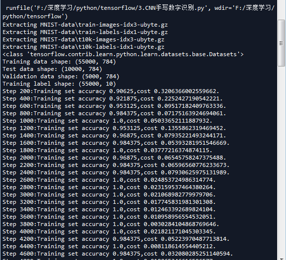
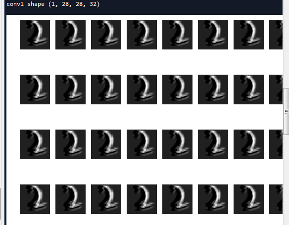
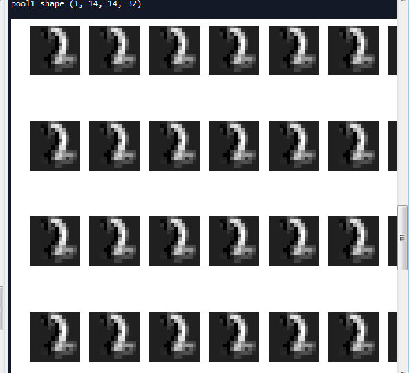
# -*- coding: utf-8 -*-
"""
Created on Mon Apr  2 18:32:47 2018

@author: Administrator
"""

'''
这里我们没有定义一个实现CNN的类,实际上我们可以定义一个CNN的类,并且把每一层也定义成一个类

利用CNN实现手写数字识别

In [1]: 导入数据,即测试集和验证集

In [2]: 引入 tensorflow 启动InteractiveSession(比session更灵活)

In [3]: 定义两个初始化w和b的函数,方便后续操作

In [4]: 定义卷积和池化函数,这里卷积采用padding,使得输入输出图像一样大,池化采取2x2,那么就是4格变一格

In [5]: 分配输入x_和y_

In [6]: 修改x的shape

In [7]: 定义第一层卷积的w和b

In [8]: 把x_image和w进行卷积,加上b,然后应用ReLU激活函数,最后进行max-pooling

In [9]: 第二层卷积,和第一层卷积类似

In [10]: 全连接层

In [11]: 为了减少过拟合,可以在输出层之前加入dropout。(但是本例子比较简单,即使不加,影响也不大)

In [12]: 由一个softmax层来得到输出

In [13]: 定义代价函数,训练步骤,用Adam来进行优化

In [14]: 使用测试集样本进行测试

'''


import tensorflow as tf
import numpy as np

'''
一 导入数据
'''
from tensorflow.examples.tutorials.mnist import input_data

#mnist是一个轻量级的类,它以numpy数组的形式存储着训练,校验,测试数据集  one_hot表示输出二值化后的10维
mnist = input_data.read_data_sets('MNIST-data',one_hot=True)

print(type(mnist)) #<class 'tensorflow.contrib.learn.python.learn.datasets.base.Datasets'>

print('Training data shape:',mnist.train.images.shape)           #Training data shape: (55000, 784)
print('Test data shape:',mnist.test.images.shape)                #Test data shape: (10000, 784)
print('Validation data shape:',mnist.validation.images.shape)    #Validation data shape: (5000, 784)
print('Training label shape:',mnist.train.labels.shape)          #Training label shape: (55000, 10)


#设置tensorflow对GPU使用按需分配
config = tf.ConfigProto()
config.gpu_options.allow_growth = True

sess = tf.InteractiveSession(config=config)


'''
二 构建网络
'''
'''
初始化权值和偏重
为了创建这个模型,我们需要创建大量的权重和偏置项。这个模型中的权重在初始化时应该加入少量的噪声来
打破对称性以及避免0梯度。由于我们使用的是ReLU神经元,因此比较好的做法是用一个较小的正数来初始化
偏置项,以避免神经元节点输出恒为0的问题(dead neurons)。为了不在建立模型的时候反复做初始化操作
,我们定义两个函数用于初始化。
'''
def weight_variable(shape):
    #使用正太分布初始化权值
    initial = tf.truncated_normal(shape,stddev=0.1)    #标准差为0.1
    return tf.Variable(initial)

def bias_variable(shape):
    initial = tf.constant(0.1,shape=shape)
    return tf.Variable(initial)

'''
卷积层和池化层
TensorFlow在卷积和池化上有很强的灵活性。我们怎么处理边界?步长应该设多大?在这个实例里,我们会
一直使用vanilla版本。我们的卷积使用1步长(stride size),0边距(padding size)的模板,保证输
出和输入是同一个大小。我们的池化用简单传统的2x2大小的模板做max pooling。为了代码更简洁,我们把
这部分抽象成一个函数。
'''
#定义卷积层
def conv2d(x,W):
    '''默认 strides[0] = strides[3] = 1,strides[1]为x方向步长,strides[2]为y方向步长
     Given an input tensor of shape `[batch, in_height, in_width, in_channels]`
     and a filter / kernel tensor of shape `[filter_height, filter_width, in_channels,
     out_channels]`
    '''
    return tf.nn.conv2d(x,W,strides=[1,1,1,1],padding = 'SAME')

#pooling层
def max_pooling(x):
    return tf.nn.max_pool(x,ksize=[1,2,2,1],strides=[1,2,2,1],padding='SAME')


#我们通过为输入图像和目标输出类别创建节点,来开始构建计算题  None表示数值不固定,用来指定batch的大小
x_ = tf.placeholder(tf.float32,[None,784])
y_ = tf.placeholder(tf.float32,[None,10])


#把x转换为卷积所需要的形式  batch_size张手写数字,每张维度为1x28x28
'''
为了用这一层,我们把x变成一个4d向量,其第2、第3维对应图片的高、高,最后一维代表图片的颜色通道数
(因为是灰度图所以这里的通道数为1,如果是rgb彩色图,则为3)。
'''
X = tf.reshape(x_,shape=[-1,28,28,1])


'''
现在我们可以开始实现第一层了。它由一个卷积接一个max pooling完成。卷积在每个5x5的patch中算出
32个特征。卷积的权重张量形状是[5, 5, 1, 32],前两个维度是patch的大小,接着是输入的通道数目,
最后是输出的通道数目。 而对于每一个输出通道都有一个对应的偏置量。
'''
#第一层卷积,32个过滤器,共享权重矩阵为1*5*5  h_conv1.shape=[-1,28,28,32]
w_conv1 = weight_variable([5,5,1,32])
b_conv1 = bias_variable([32])
h_conv1 = tf.nn.relu(conv2d(X,w_conv1) + b_conv1)

#第一个pooling层 最大值池化层2x2 [-1,28,28,28]->[-1,14,14,32]
h_pool1 = max_pooling(h_conv1)


#第二层卷积,64个过滤器,共享权重矩阵为32*5*5  h_conv2.shape=[-1,14,14,64]
w_conv2 = weight_variable([5,5,32,64])
b_conv2 = bias_variable([64])
h_conv2 = tf.nn.relu(conv2d(h_pool1,w_conv2) + b_conv2)

#第二个pooling层 最大值池化层2x2 [-1,14,14,64]->[-1,7,7,64]
h_pool2 = max_pooling(h_conv2)

'''
全连接层
现在,图片尺寸减小到7x7,我们加入一个有1024个神经元的全连接层,用于处理整个图片。我们把池化层输
出的张量reshape成一些向量,乘上权重矩阵,加上偏置,然后对其使用ReLU。
'''
h_poo2_falt = tf.reshape(h_pool2,[-1,7*7*64])
#隐藏层
w_h = weight_variable([7*7*64,1024])
b_h = bias_variable([1024])
hidden = tf.nn.relu(tf.matmul(h_poo2_falt,w_h) + b_h)


'''
加入弃权,把部分神经元输出置为0
为了减少过拟合,我们在输出层之前加入dropout。我们用一个placeholder来代表一个神经元的输出在
dropout中保持不变的概率。这样我们可以在训练过程中启用dropout,在测试过程中关闭dropout。
TensorFlow的tf.nn.dropout操作除了可以屏蔽神经元的输出外,还会自动处理神经元输出值的scale。
所以用dropout的时候可以不用考虑scale。
'''
keep_prob = tf.placeholder(tf.float32)    #弃权概率0.0-1.0  1.0表示不使用弃权
hidden_drop = tf.nn.dropout(hidden,keep_prob)

'''
输出层
最后,我们添加一个softmax层,就像前面的单层softmax regression一样。
'''
w_o = weight_variable([1024,10])
b_o = bias_variable([10])
output = tf.nn.softmax(tf.matmul(hidden_drop,w_o) + b_o)


'''
三 设置对数似然损失函数
'''
#代价函数 J =-(Σy.logaL)/n    .表示逐元素乘
cost = tf.reduce_mean(-tf.reduce_sum(y_*tf.log(output),axis=1))


'''
四 求解
'''
train = tf.train.AdamOptimizer(0.0001).minimize(cost)

#预测结果评估
#tf.argmax(output,1)  按行统计最大值得索引
correct = tf.equal(tf.argmax(output,1),tf.argmax(y_,1))       #返回一个数组 表示统计预测正确或者错误
accuracy = tf.reduce_mean(tf.cast(correct,tf.float32))        #求准确率


#创建list 保存每一迭代的结果
training_accuracy_list = []
test_accuracy_list = []
training_cost_list=[]
test_cost_list=[]


#使用会话执行图
sess.run(tf.global_variables_initializer())   #初始化变量


#开始迭代 使用Adam优化的随机梯度下降法
for i in range(5000):   #一个epoch需要迭代次数计算公式:测试集长度 / batch_size
    x_batch,y_batch = mnist.train.next_batch(batch_size = 64)
    #开始训练
    train.run(feed_dict={x_:x_batch,y_:y_batch,keep_prob:1.0})
    if (i+1)%200 == 0:
         #输出训练集准确率
        #training_accuracy = accuracy.eval(feed_dict={x_:mnist.train.images,y_:mnist.train.labels})
        training_accuracy,training_cost = sess.run([accuracy,cost],feed_dict={x_:x_batch,y_:y_batch,keep_prob:1.0})
        training_accuracy_list.append(training_accuracy)
        training_cost_list.append(training_cost)
        print('Step {0}:Training set accuracy {1},cost {2}.'.format(i+1,training_accuracy,training_cost))

#全部训练完成做测试  分成200次,一次测试50个样本
#输出测试机准确率   如果一次性全部做测试,内容不够用会出现OOM错误。所以测试时选取比较小的mini_batch来测试
#test_accuracy = accuracy.eval(feed_dict={x_:mnist.test.images,y_:mnist.test.labels})
for i in range(200):
    x_batch,y_batch = mnist.test.next_batch(batch_size = 50)
    test_accuracy,test_cost = sess.run([accuracy,cost],feed_dict={x_:x_batch,y_:y_batch,keep_prob:1.0})
    test_accuracy_list.append(test_accuracy)
    test_cost_list.append(test_cost)
    if (i+1)%20 == 0:
         print('Step {0}:Test set accuracy {1},cost {2}.'.format(i+1,test_accuracy,test_cost))
print('Test accuracy:',np.mean(test_accuracy_list))


'''
图像操作
'''
import matplotlib.pyplot as plt
#随便取一张图像
img = mnist.train.images[2]
label = mnist.train.labels[2]

#print('图像像素值:{0},对应的标签{1}'.format(img.reshape(28,28),np.argmax(label)))
print('图像对应的标签{0}'.format(np.argmax(label)))

plt.figure()

#子图1
plt.subplot(1,2,1)
plt.imshow(img.reshape(28,28))                #显示的是热度图片
plt.axis('off')                               #不显示坐标轴

#子图2
plt.subplot(1,2,2)
plt.imshow(img.reshape(28,28),cmap='gray')    #显示灰度图片
plt.axis('off')


plt.show()

'''
显示卷积和池化层结果
'''
plt.figure(figsize=(1.0*8,1.6*4))
plt.subplots_adjust(bottom=0,left=.01,right=.99,top=.90,hspace=.35)
#显示第一个卷积层之后的结果  (1,28,28,32)
conv1 = h_conv1.eval(feed_dict={x_:img.reshape([-1,784]),y_:label.reshape([-1,10]),keep_prob:1.0})
print('conv1 shape',conv1.shape)

for i in range(32):
    show_image = conv1[:,:,:,1]
    show_image.shape = [28,28]
    plt.subplot(4,8,i+1)
    plt.imshow(show_image,cmap='gray')
    plt.axis('off')
plt.show()

plt.figure(figsize=(1.2*8,2.0*4))
plt.subplots_adjust(bottom=0,left=.01,right=.99,top=.90,hspace=.35)
#显示第一个池化层之后的结果  (1,14,14,32)
pool1 = h_pool1.eval(feed_dict={x_:img.reshape([-1,784]),y_:label.reshape([-1,10]),keep_prob:1.0})
print('pool1 shape',pool1.shape)

for i in range(32):
    show_image = pool1[:,:,:,1]
    show_image.shape = [14,14]
    plt.subplot(4,8,i+1)
    plt.imshow(show_image,cmap='gray')
    plt.axis('off')
plt.show()
运行结果如下