第九节，线性逻辑回归

一般来说，回归不用在分类问题上，因为回归是连续型模型，而且受噪声影响比较大。如果非要应用进入，可以使用logistic回归。logistic回归本质上是线性回归，只是在特征到结果的映射中加入了一层函数映射，即先把特征线性求和，然后使用函数g(z)函数来预测。

下面介绍一个线性逻辑回归的案例，这里被用来处理二分类和多分类问题。

一 实例描述

假设某肿瘤医院想用神经网络对已有的病例数据进行分类，数据的样本特征包括病人的年龄和肿瘤的大小，对应的标签为病例是良性肿瘤还是恶性肿瘤。

二 二分类问题

1.生成样本集

因为这里没有医院的病例数据，为了方便演示，使用python生成一些模拟数据来替代样本，它应该是二维的数组"年龄，肿瘤大小"，generate()函数为生成模拟样本的函数，意思是按照指定的均值和方差生成固定数量的样本。

def get_one_hot(labels,num_classes):
    '''
    one_hot编码
    
    args:
        labels : 输如类标签
        num_classes：类别个数
    '''    
    m = np.zeros([labels.shape[0],num_classes])
    for i in range(labels.shape[0]):  
        m[i][labels[i]] = 1
    return m
        
    

def  generate(sample_size,mean,cov,diff,num_classes=2,one_hot = False):
    '''
    因为没有医院的病例数据，所以模拟生成一些样本
    按照指定的均值和方差生成固定数量的样本
    
    args:
        sample_size:样本个数
        mean: 长度为 M 的 一维ndarray或者list  对应每个特征的均值
        cov： N X N的ndarray或者list  协方差  对称矩阵
        diff:长度为 类别-1 的list    每i元素为第i个类别和第0个类别均值的差值 [特征1差，特征2差....]  如果长度不够，后面每个元素值取diff最后一个元素
        num_classes：分类数
        one_hot : one_hot编码
    '''
        
    #每一类的样本数 假设有1000个样本 分两类，每类500个样本    
    sample_per_class = int(sample_size/num_classes)
    
    
    '''
    多变量正态分布
    mean : 1-D array_like, of length N . Mean of the N-dimensional distribution.    数组类型，每一个元素对应一维的平均值
    cov : 2-D array_like, of shape (N, N) .Covariance matrix of the distribution. It must be symmetric and positive-semidefinite 
        for proper sampling.
    size:shape. Given a shape of, for example, (m,n,k), m*n*k samples are generated, and packed in an m-by-n-by-k arrangement.
        Because each sample is N-dimensional, the output shape is (m,n,k,N). If no shape is specified, a single (N-D) sample is 
        returned.
    '''
    #生成均值为mean,协方差为cov sample_per_class x len(mean)个样本 类别为0
    X0 = np.random.multivariate_normal(mean,cov,sample_per_class)    
    Y0 = np.zeros(sample_per_class,dtype=np.int32)
    
    
    #对于diff长度不够进行处理
    if len(diff) != num_classes-1:
        tmp = np.zeros(num_classes-1)
        tmp[0:len(diff)] = diff  
        tmp[len(diff):] = diff[-1]
    else:
        tmp = diff
    
    
    for ci,d  in enumerate(tmp):
        '''
        把list变成 索引-元素树，同时迭代索引和元素本身
        '''
        
        #生成均值为mean+d,协方差为cov sample_per_class x len(mean)个样本 类别为ci+1
        X1 = np.random.multivariate_normal(mean+d,cov,sample_per_class)                
        Y1 = (ci+1)*np.ones(sample_per_class,dtype=np.int32)
                
        #合并X0,X1  按列拼接
        X0 = np.concatenate((X0,X1))
        Y0 = np.concatenate((Y0,Y1))
        
        
    if one_hot:           
        Y0 = get_one_hot(Y0,num_classes)
        
    #打乱顺序
    X,Y  =  shuffle(X0,Y0)
    
    return X,Y

下面代码是调用该函数生成100个样本，并将它们可视化

• 定义水机数的种子值，这样每次运行代码时生成的随机值都是一样的。
• generate()函数中传入的[3.0]表示两类数据x,y差距是3.0。传入最后一个参数one_hot=False表示不使用one_hot编码。

    '''
    生成随机数据
    '''
    np.random.seed(10)
    #特征个数
    num_features = 2
    #样本个数
    num_samples = 100
    #n返回长度为特征的数组 正太分布
    mean = np.random.randn(num_features)
    print('mean',mean)
    cov = np.eye(num_features)
    print('cov',cov)
    X,Y = generate(num_samples,mean,cov,[3.0],num_classes=2)
    #print('X',X)
    #print('Y',Y)
    colors = ['r' if l == 0 else 'b'  for l in Y[:]]
    plt.scatter(X[:,0],X[:,1],c=colors)
    plt.xlabel('Scaled age (in yrs)')
    plt.ylabel('Tumor size (in cm)')
    
    
    #输出维度
    lab_dim = 1

 2 构建网络结构

• 构建网络结构，使用一个神经元，先定义输入、输出两个占位符，然后是w和b的值。
• 使用sigmoid激活函数。
• 定义sigmoid交叉熵代价函数。
• 使用AdamOptimizer优化器。

 构建网络结构
    '''

    #构建输入占位符
    input_x = tf.placeholder(dtype = tf.float32,shape = [None,num_features])
    input_y = tf.placeholder(dtype = tf.float32,shape = [None,lab_dim])
    
    #定义学习参数
    W = tf.Variable(tf.truncated_normal(shape=[num_features,lab_dim]),name = 'weight')
    b = tf.Variable(tf.zeros([lab_dim]),name='bias')
    
    
    #定义输出
    output = tf.nn.sigmoid(tf.matmul(input_x,W) + b)
    print(output.get_shape().as_list())
    
    '''
    #定义了两个不同的代价函数
    '''
    #定义sigmoid交叉熵
    cost = tf.reduce_mean( -(input_y*tf.log(output) + (1-input_y)*tf.log(1-output)))
    #最二次代价函数
    loss = tf.reduce_mean(tf.square(input_y - output))
    
    #尽量用这个 收敛速度更快 
    train = tf.train.AdamOptimizer(0.04).minimize(cost)

3 训练并可视化显示

 #设置参数进行训练
    training_epochs = 50
    batch_size = 32
    
    with tf.Session() as sess:
        #初始化变量
        sess.run(tf.global_variables_initializer())
    
        training_data = list(zip(X,Y))   
        #开始迭代
        for epoch in range(training_epochs):    
            random.shuffle(training_data)    
            mini_batchs = [training_data[k:k+batch_size] for k in range(0,num_samples,batch_size)]
            
            #总的代价
            cost_list = []
            for mini_batch in mini_batchs:
                x_batch = np.asarray([x  for x,y in mini_batch ] ,dtype=np.float32).reshape(-1,num_features)                                                  
                y_batch = np.asarray([y  for x,y in mini_batch ] ,dtype=np.float32).reshape(-1,lab_dim)                                   
                _,lossval = sess.run([train,loss],feed_dict={input_x:x_batch,input_y:y_batch})
                cost_list.append(lossval)
                
        
            print('Epoch {0}  cost  {1}'.format(epoch,np.mean(cost_list)))
            
            
        #绘制z= w1x1 + w2x2 + b = 0的分界线
        x = np.linspace(-1,8,200)
        y = -x*( sess.run(W)[0] / sess.run(W)[1]) - sess.run(b)/sess.run(W)[1]
        plt.plot(x,y,label='Filtted line')
        plt.legend()
        plt.show()

由于输入特征个数为两个，所以模型生成的z用公式可以表示成z=w1x1 + w2x2 +b。如果将x1和x2映射映射到直角坐标系中的x和y坐标，那么z就可以被分为大于0和小于0两部分。当z=0时，就代表直线本身。令z=0，就可以将模型转换为如下直线方程：

x2 = -x1*w1/w2 - b/w2   即: y= -x*(w1/w2) - b/w2

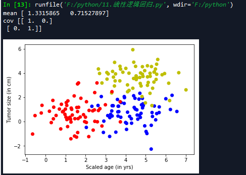
线性可分：如上图所示，可以用直线分割的方式解决问题，则可以说这个问题是线性可分的。

三 多分类问题

还是接着上面的例子，这次在数据集中再添加一类样本，可以使用多条直线将数据分成多类。

1 生成样本集

'''
    生成随机数据
    '''
    np.random.seed(10)
    #特征个数
    num_features = 2
    #样本个数
    num_samples = 200
    #n返回长度为特征的数组 正太分布
    mean = np.random.randn(num_features)
    print('mean',mean)
    cov = np.eye(num_features)
    print('cov',cov)
    train_x,train_y = generate(num_samples,mean,cov,[[3.0,0.0],[3.0,3.0]],num_classes=3,one_hot = True)
    #print('X',X)
    #print('Y',Y)
    train_labels = [np.argmax(l) for l in train_y]     
    color = ['r','b','y']
    colors = [color[l]  for l in train_labels[:]]
    plt.scatter(train_x[:,0],train_x[:,1],c=colors)
    plt.xlabel('Scaled age (in yrs)')
    plt.ylabel('Tumor size (in cm)')
    
    
    #输出维度
    lab_dim = 3

 2 构建网络结构

    '''
    构建网络结构
    '''
    
    #构建输入占位符
    input_x = tf.placeholder(dtype = tf.float32,shape = [None,num_features])
    input_y = tf.placeholder(dtype = tf.float32,shape = [None,lab_dim])
    
    #定义学习参数
    W = tf.Variable(tf.truncated_normal(shape=[num_features,lab_dim]),name = 'weight')
    b = tf.Variable(tf.zeros([lab_dim]),name='bias')
    
    
    
    #定义输出
    logits = tf.matmul(input_x,W) + b
    output =  tf.nn.softmax(logits)
        
    output_labels = tf.argmax(output,axis=1)
    print(output.get_shape().as_list())
        
    '''
    定义了两个不同的代价函数
    '''
    #定义softmax交叉熵
    cost = tf.reduce_mean( tf.nn.softmax_cross_entropy_with_logits(labels = input_y,logits = logits))
        
    #尽量用这个 收敛速度更快 
    train = tf.train.AdamOptimizer(0.04).minimize(cost)

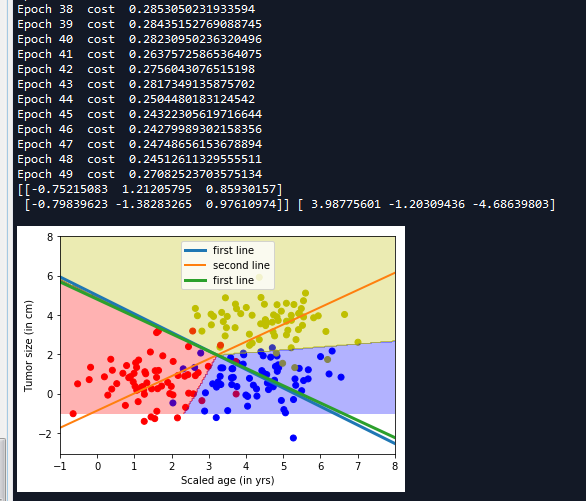
3 训练并可视化显示

 #设置参数进行训练
    training_epochs = 50
    batch_size = 32
    
    with tf.Session() as sess:
        #初始化变量
        sess.run(tf.global_variables_initializer())
    
        training_data = list(zip(train_x,train_y))   
        #开始迭代
        for epoch in range(training_epochs):    
            random.shuffle(training_data)    
            mini_batchs = [training_data[k:k+batch_size] for k in range(0,num_samples,batch_size)]
            
            #总的代价
            cost_list = []
            for mini_batch in mini_batchs:
                x_batch = np.asarray([x  for x,y in mini_batch ] ,dtype=np.float32).reshape(-1,num_features)                                                  
                y_batch = np.asarray([y  for x,y in mini_batch ] ,dtype=np.float32).reshape(-1,lab_dim)                                   
                _,lossval = sess.run([train,cost],feed_dict={input_x:x_batch,input_y:y_batch})
                cost_list.append(lossval)
                
        
            print('Epoch {0}  cost  {1}'.format(epoch,np.mean(cost_list)))
            
        '''
        数据可视化
        '''      
        x = np.linspace(-1,8,200)
        
        y = -x*(sess.run(W)[0][0]/sess.run(W)[1][0]) - sess.run(b)[0]/sess.run(W)[1][0]
        plt.plot(x,y,label = 'first line',lw = 3)
    
    
        y = -x*(sess.run(W)[0][1]/sess.run(W)[1][1]) - sess.run(b)[1]/sess.run(W)[1][1]
        plt.plot(x,y,label = 'second line',lw = 2)
        
        y = -x*(sess.run(W)[0][2]/sess.run(W)[1][2]) - sess.run(b)[2]/sess.run(W)[1][2]
        plt.plot(x,y,label = 'first line',lw = 3)
        
        plt.legend()
        print(sess.run(W),sess.run(b))
        
        
        
        nb_of_xs = 200
        xs1 = np.linspace(-1,8,num = nb_of_xs)
        xs2 = np.linspace(-1,8,num = nb_of_xs)
        
        #创建网格
        xx,yy = np.meshgrid(xs1,xs2)
        
        #初始化和填充 classfication plane
        classfication_plane = np.zeros([nb_of_xs,nb_of_xs])
        
        for i in range(nb_of_xs):
            for j in range(nb_of_xs):
                #计算每个输入样本对应的分类标签
                classfication_plane[i,j] = sess.run(output_labels,feed_dict={input_x:[[xx[i,j],yy[i,j]]]})
                
        #创建 color map用于显示
        cmap = ListedColormap([
                    colorConverter.to_rgba('r',alpha = 0.30),
                    colorConverter.to_rgba('b',alpha = 0.30),
                    colorConverter.to_rgba('y',alpha = 0.30)
                ])
        #显示各个样本边界
        plt.contourf(xx,yy,classfication_plane,cmap = cmap)
        plt.show()

完整代码：

# -*- coding: utf-8 -*-
"""
Created on Mon Apr 23 17:33:32 2018

@author: zy
"""

import  numpy   as  np
import  tensorflow as tf
from sklearn.utils import shuffle
import matplotlib.pyplot as plt
import random
from matplotlib.colors import colorConverter, ListedColormap 




'''
线性逻辑可分 对肿瘤病例进行分类 样本特征包括病人的年龄和肿瘤的大小
像下面程序所示的可以用直线分割的方式解决问题，则可以说这个问题是线性可分的
'''

def get_one_hot(labels,num_classes):
    '''
    one_hot编码
    
    args:
        labels : 输如类标签
        num_classes：类别个数
    '''    
    m = np.zeros([labels.shape[0],num_classes])
    for i in range(labels.shape[0]):  
        m[i][labels[i]] = 1
    return m
        
    

def  generate(sample_size,mean,cov,diff,num_classes=2,one_hot = False):
    '''
    因为没有医院的病例数据，所以模拟生成一些样本
    按照指定的均值和方差生成固定数量的样本
    
    args:
        sample_size:样本个数
        mean: 长度为 M 的 一维ndarray或者list  对应每个特征的均值
        cov： N X N的ndarray或者list  协方差  对称矩阵
        diff:长度为 类别-1 的list    每i元素为第i个类别和第0个类别均值的差值 [特征1差，特征2差....]  如果长度不够，后面每个元素值取diff最后一个元素
        num_classes：分类数
        one_hot : one_hot编码
    '''
        
    #每一类的样本数 假设有1000个样本 分两类，每类500个样本    
    sample_per_class = int(sample_size/num_classes)
    
    
    '''
    多变量正态分布
    mean : 1-D array_like, of length N . Mean of the N-dimensional distribution.    数组类型，每一个元素对应一维的平均值
    cov : 2-D array_like, of shape (N, N) .Covariance matrix of the distribution. It must be symmetric and positive-semidefinite 
        for proper sampling.
    size:shape. Given a shape of, for example, (m,n,k), m*n*k samples are generated, and packed in an m-by-n-by-k arrangement.
        Because each sample is N-dimensional, the output shape is (m,n,k,N). If no shape is specified, a single (N-D) sample is 
        returned.
    '''
    #生成均值为mean,协方差为cov sample_per_class x len(mean)个样本 类别为0
    X0 = np.random.multivariate_normal(mean,cov,sample_per_class)    
    Y0 = np.zeros(sample_per_class,dtype=np.int32)
    
    
    #对于diff长度不够进行处理
    if len(diff) != num_classes-1:
        tmp = np.zeros(num_classes-1)
        tmp[0:len(diff)] = diff  
        tmp[len(diff):] = diff[-1]
    else:
        tmp = diff
    
    
    for ci,d  in enumerate(tmp):
        '''
        把list变成 索引-元素树，同时迭代索引和元素本身
        '''
        
        #生成均值为mean+d,协方差为cov sample_per_class x len(mean)个样本 类别为ci+1
        X1 = np.random.multivariate_normal(mean+d,cov,sample_per_class)                
        Y1 = (ci+1)*np.ones(sample_per_class,dtype=np.int32)
                
        #合并X0,X1  按列拼接
        X0 = np.concatenate((X0,X1))
        Y0 = np.concatenate((Y0,Y1))
        
        
    if one_hot:           
        Y0 = get_one_hot(Y0,num_classes)
        
    #打乱顺序
    X,Y  =  shuffle(X0,Y0)
    
    return X,Y



def  LinearClassification():
    
    '''
    下面是一个线性二分类问题
    '''
    
    '''
    生成随机数据
    '''
    np.random.seed(10)
    #特征个数
    num_features = 2
    #样本个数
    num_samples = 100
    #n返回长度为特征的数组 正太分布
    mean = np.random.randn(num_features)
    print('mean',mean)
    cov = np.eye(num_features)
    print('cov',cov)
    X,Y = generate(num_samples,mean,cov,[3.0],num_classes=2)
    #print('X',X)
    #print('Y',Y)
    colors = ['r' if l == 0 else 'b'  for l in Y[:]]
    plt.scatter(X[:,0],X[:,1],c=colors)
    plt.xlabel('Scaled age (in yrs)')
    plt.ylabel('Tumor size (in cm)')
    
    
    #输出维度
    lab_dim = 1
    '''
    构建网络结构
    '''

    #构建输入占位符
    input_x = tf.placeholder(dtype = tf.float32,shape = [None,num_features])
    input_y = tf.placeholder(dtype = tf.float32,shape = [None,lab_dim])
    
    #定义学习参数
    W = tf.Variable(tf.truncated_normal(shape=[num_features,lab_dim]),name = 'weight')
    b = tf.Variable(tf.zeros([lab_dim]),name='bias')
    
    
    #定义输出
    output = tf.nn.sigmoid(tf.matmul(input_x,W) + b)
    print(output.get_shape().as_list())
    
    '''
    #定义了两个不同的代价函数
    '''
    #定义sigmoid交叉熵
    cost = tf.reduce_mean( -(input_y*tf.log(output) + (1-input_y)*tf.log(1-output)))
    #最二次代价函数
    loss = tf.reduce_mean(tf.square(input_y - output))
    
    #尽量用这个 收敛速度更快 
    train = tf.train.AdamOptimizer(0.04).minimize(cost)
    
    
    #设置参数进行训练
    training_epochs = 50
    batch_size = 32
    
    with tf.Session() as sess:
        #初始化变量
        sess.run(tf.global_variables_initializer())
    
        training_data = list(zip(X,Y))   
        #开始迭代
        for epoch in range(training_epochs):    
            random.shuffle(training_data)    
            mini_batchs = [training_data[k:k+batch_size] for k in range(0,num_samples,batch_size)]
            
            #总的代价
            cost_list = []
            for mini_batch in mini_batchs:
                x_batch = np.asarray([x  for x,y in mini_batch ] ,dtype=np.float32).reshape(-1,num_features)                                                  
                y_batch = np.asarray([y  for x,y in mini_batch ] ,dtype=np.float32).reshape(-1,lab_dim)                                   
                _,lossval = sess.run([train,loss],feed_dict={input_x:x_batch,input_y:y_batch})
                cost_list.append(lossval)
                
        
            print('Epoch {0}  cost  {1}'.format(epoch,np.mean(cost_list)))
            
            
        #绘制z= w1x1 + w2x2 + b = 0的分界线
        x = np.linspace(-1,8,200)
        y = -x*( sess.run(W)[0] / sess.run(W)[1]) - sess.run(b)/sess.run(W)[1]
        plt.plot(x,y,label='Filtted line')
        plt.legend()
        plt.show()


def  LinearMultiClassification():
    
    '''
    下面是一个线性多分类问题
    '''
    
    '''
    生成随机数据
    '''
    np.random.seed(10)
    #特征个数
    num_features = 2
    #样本个数
    num_samples = 200
    #n返回长度为特征的数组 正太分布
    mean = np.random.randn(num_features)
    print('mean',mean)
    cov = np.eye(num_features)
    print('cov',cov)
    train_x,train_y = generate(num_samples,mean,cov,[[3.0,0.0],[3.0,3.0]],num_classes=3,one_hot = True)
    #print('X',X)
    #print('Y',Y)
    train_labels = [np.argmax(l) for l in train_y]     
    color = ['r','b','y']
    colors = [color[l]  for l in train_labels[:]]
    plt.scatter(train_x[:,0],train_x[:,1],c=colors)
    plt.xlabel('Scaled age (in yrs)')
    plt.ylabel('Tumor size (in cm)')
    
    
    #输出维度
    lab_dim = 3
    '''
    构建网络结构
    '''
    
    #构建输入占位符
    input_x = tf.placeholder(dtype = tf.float32,shape = [None,num_features])
    input_y = tf.placeholder(dtype = tf.float32,shape = [None,lab_dim])
    
    #定义学习参数
    W = tf.Variable(tf.truncated_normal(shape=[num_features,lab_dim]),name = 'weight')
    b = tf.Variable(tf.zeros([lab_dim]),name='bias')
    
    
    
    #定义输出
    logits = tf.matmul(input_x,W) + b
    output =  tf.nn.softmax(logits)
        
    output_labels = tf.argmax(output,axis=1)
    print(output.get_shape().as_list())
        
    '''
    定义了两个不同的代价函数
    '''
    #定义softmax交叉熵
    cost = tf.reduce_mean( tf.nn.softmax_cross_entropy_with_logits(labels = input_y,logits = logits))
        
    #尽量用这个 收敛速度更快 
    train = tf.train.AdamOptimizer(0.04).minimize(cost)
    
    
    #设置参数进行训练
    training_epochs = 50
    batch_size = 32
    
    with tf.Session() as sess:
        #初始化变量
        sess.run(tf.global_variables_initializer())
    
        training_data = list(zip(train_x,train_y))   
        #开始迭代
        for epoch in range(training_epochs):    
            random.shuffle(training_data)    
            mini_batchs = [training_data[k:k+batch_size] for k in range(0,num_samples,batch_size)]
            
            #总的代价
            cost_list = []
            for mini_batch in mini_batchs:
                x_batch = np.asarray([x  for x,y in mini_batch ] ,dtype=np.float32).reshape(-1,num_features)                                                  
                y_batch = np.asarray([y  for x,y in mini_batch ] ,dtype=np.float32).reshape(-1,lab_dim)                                   
                _,lossval = sess.run([train,cost],feed_dict={input_x:x_batch,input_y:y_batch})
                cost_list.append(lossval)
                
        
            print('Epoch {0}  cost  {1}'.format(epoch,np.mean(cost_list)))
            
        '''
        数据可视化
        '''      
        x = np.linspace(-1,8,200)
        
        y = -x*(sess.run(W)[0][0]/sess.run(W)[1][0]) - sess.run(b)[0]/sess.run(W)[1][0]
        plt.plot(x,y,label = 'first line',lw = 3)
    
    
        y = -x*(sess.run(W)[0][1]/sess.run(W)[1][1]) - sess.run(b)[1]/sess.run(W)[1][1]
        plt.plot(x,y,label = 'second line',lw = 2)
        
        y = -x*(sess.run(W)[0][2]/sess.run(W)[1][2]) - sess.run(b)[2]/sess.run(W)[1][2]
        plt.plot(x,y,label = 'first line',lw = 3)
        
        plt.legend()
        print(sess.run(W),sess.run(b))
        
        
        
        nb_of_xs = 200
        xs1 = np.linspace(-1,8,num = nb_of_xs)
        xs2 = np.linspace(-1,8,num = nb_of_xs)
        
        #创建网格
        xx,yy = np.meshgrid(xs1,xs2)
        
        #初始化和填充 classfication plane
        classfication_plane = np.zeros([nb_of_xs,nb_of_xs])
        
        for i in range(nb_of_xs):
            for j in range(nb_of_xs):
                #计算每个输入样本对应的分类标签
                classfication_plane[i,j] = sess.run(output_labels,feed_dict={input_x:[[xx[i,j],yy[i,j]]]})
                
        #创建 color map用于显示
        cmap = ListedColormap([
                    colorConverter.to_rgba('r',alpha = 0.30),
                    colorConverter.to_rgba('b',alpha = 0.30),
                    colorConverter.to_rgba('y',alpha = 0.30)
                ])
        #显示各个样本边界
        plt.contourf(xx,yy,classfication_plane,cmap = cmap)
        plt.show()
        
if __name__== '__main__':
    LinearMultiClassification()
    #LinearClassification()