#聚类分析
par(mfrow=c(1,1))
#计算距离
install.packages("flexclust")
data(nutrient,package="flexclust")
head(nutrient,4)
energy protein fat calcium iron
beef braised 340 20 28 9 2.6
hamburger 245 21 17 9 2.7
beef roast 420 15 39 7 2.0
beef steak 375 19 32 9 2.6
d<-dist(nutrient)
as.matrix(d)[1:4,1:4]
beef braised hamburger beef roast beef steak
beef braised 0.00000 95.6400 80.93429 35.24202
hamburger 95.64000 0.0000 176.49218 130.87784
beef roast 80.93429 176.4922 0.00000 45.76418
beef steak 35.24202 130.8778 45.76418 0.00000
#层次聚类分析
par(nfrow=c(1,1))
data(nutrient,package="flexclust")
row.names(nutrient)<-tolower(row.names(nutrient))
nutrient.scaled<-scale(nutrient)
d<-dist(nutrient.scaled)
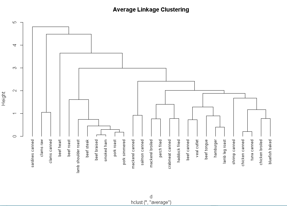
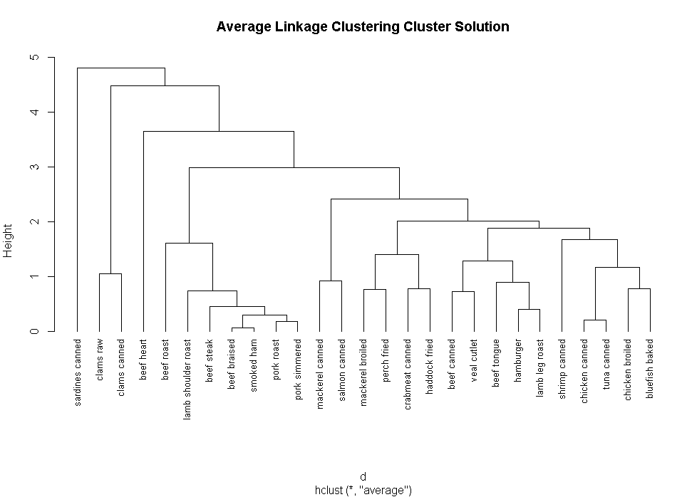
fit.average<-hclust(d,method="average")
plot(fit.average,hang=-1,cex=.8,main="Average Linkage Clustering")
#选择聚类的个数
install.packages("NbClust")
library(NbClust)
devAskNewPage(ask=TRUE)
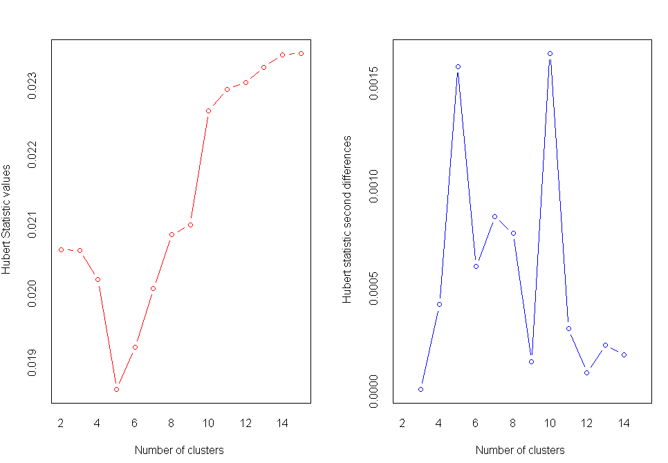
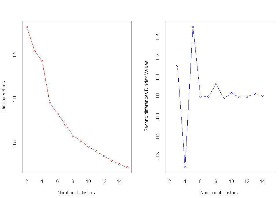
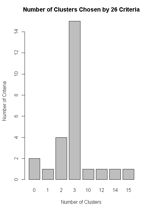
nc<-NbClust(nutrient.scaled,distance="euclidean",min.nc=2,max.nc=15,method="average")
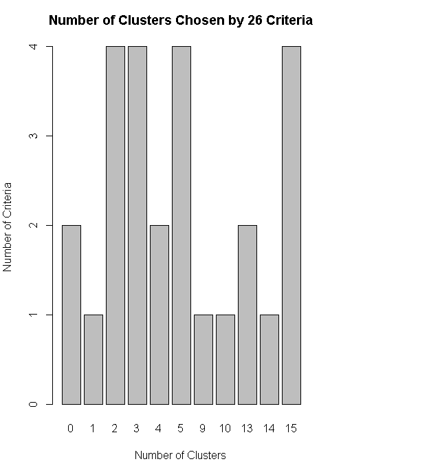
table(nc$Best.n[1,])
barplot(table(nc$Best.n[1,]),xlab="Number of Clusters",ylab="Number of Criteria",main="Number of Clusters Chosen by 26 Criteria")
#获取最终的聚类方案
par(mfrow=c(1,1))
clusters<-cutree(fit.average,k=5)
table(clusters)
1 2 3 4 5
7 16 1 2 1
aggregate(nutrient,by=list(cluster=clusters),median)
cluster energy protein fat calcium iron
1 1 340.0 19 29 9 2.50
2 2 170.0 20 8 13 1.45
3 3 160.0 26 5 14 5.90
4 4 57.5 9 1 78 5.70
5 5 180.0 22 9 367 2.50
aggregate(as.data.frame(nutrient.scaled),by=list(cluster=clusters),median)
cluster energy protein fat calcium iron
1 1 1.3101024 0.0000000 1.3785620 -0.4480464 0.08110456
2 2 -0.3696099 0.2352002 -0.4869384 -0.3967868 -0.63743114
3 3 -0.4684165 1.6464016 -0.7534384 -0.3839719 2.40779157
4 4 -1.4811842 -2.3520023 -1.1087718 0.4361807 2.27092763
5 5 -0.2708033 0.7056007 -0.3981050 4.1396825 0.08110456
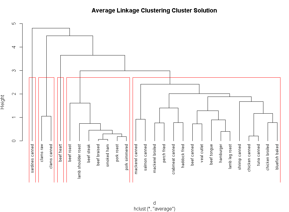
plot(fit.average,hang=-1,cex=.8,main="Average Linkage Clustering Cluster Solution")
rect.hclust(fit.average,k=5)
#划分聚类分析
install.packages("rattle")
#install.packages("RGtk2")
install.packages("https://cran.r-project.org/bin/windows/contrib/3.3/RGtk2_2.20.31.zip", repos=NULL)
install.packages("httr")
library("rattle")
library("RGtk2")
library("httr")
a <- GET("https://archive.ics.uci.edu/ml/machine-learning-databases/wine/wine.data")
wine <- read.csv(textConnection(content(a)), header=F)
names(wine)<-c("Type","Alcohol","Malic acid","Ash","Alcalinity of ash","Magnesium","Total phenols","Flavanoids","Nonflavanoid phenols","Proanthocyanins","Color intensity","Hue","OD280/OD315 of diluted wines","Proline")
#data(wine,package="rattle")
head(wine)
df<-scale(wine[-1])
wssplot(df)
library(NbClust)
set.seed(1234)
devAskNewPage(ask=TRUE)
nc<-NbClust(df,min.nc=2,max.nc=15,method="kmeans")
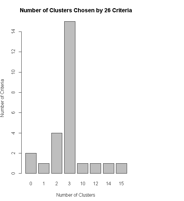
table(nc$Best.n[1,])
barplot(table(nc$Best.n[1,]),xlab="Number of Clusters",ylab="Number of Criteria",main="Number of Clusters Chosen by 26 Criteria")
set.seed(1234)
fit.km<-kmeans(df,3,nstart=25)
fit.km$size
fit.km$centers
ct.km<-table(wine$Type,fit.km$cluster)
ct.km
1 2 3
1 59 0 0
2 3 65 3
3 0 0 48
library(flexclust)
randIndex(ct.km)
ARI
0.897495
#围绕中心点的划分
library(cluster)
set.seed(1234)
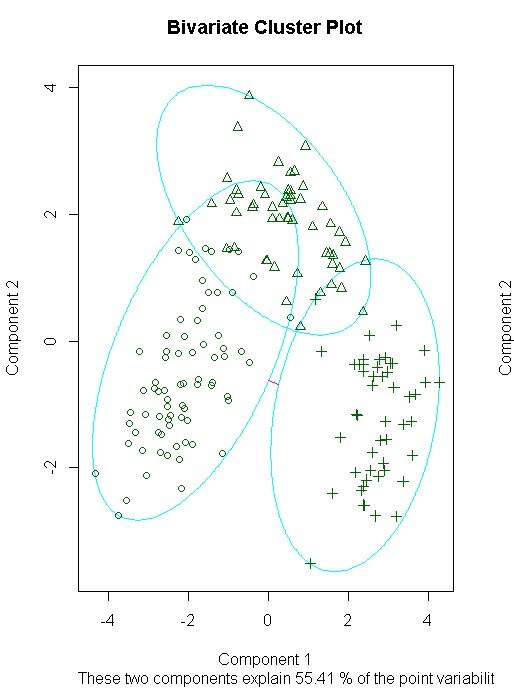
fit.pam<-pam(wine[-1],k=3,stand=TRUE)
fit.pam$method
clusplot(fit.pam,main="Bivariate Cluster Plot")
library(flexclust)
randIndex(ct.pam)
ARI
0.6994957
#围绕中心点的划分
library(cluster)
set.seed(1234)
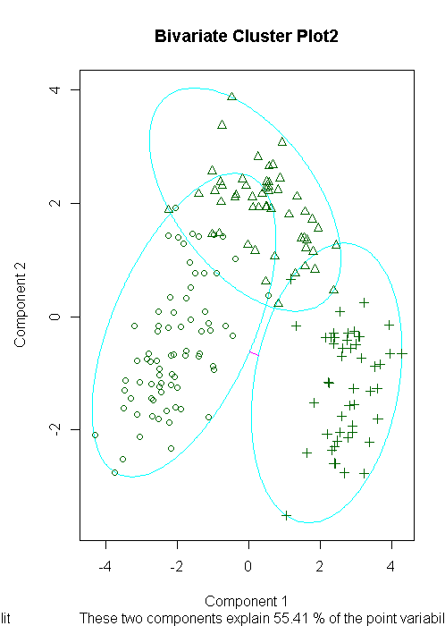
fit.pam<-pam(wine[-1],k=3,stand=TRUE)
fit.pam$medoids
clusplot(fit.pam,main="Bivariate Cluster Plot2")
ct.pam<-table(wine$Type,fit.pam$clustering)
randIndex(ct.pam)
ARI
0.6994957
#避免不存在的类
install.packages("fMultivar")
library(fMultivar)
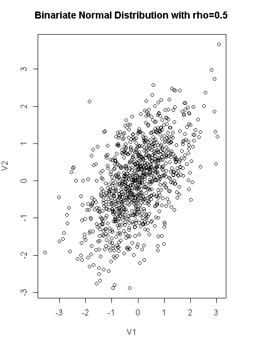
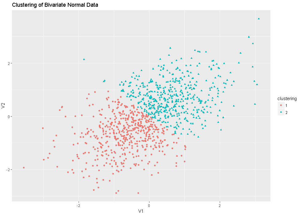
set.seed(1234)
df<-rnorm2d(1000,rho=.5)
df<-as.data.frame(df)
plot(df,main="Binariate Normal Distribution with rho=0.5")
#wssplot(df)
library(NbClust)
nc<-NbClust(df,min.nc=2,max.nc=15,method="kmeans")
dev.new()
barplot(table(nc$Best.n[1,]),xlab="Number of Clusters",ylab="Number of Criteria",main="Number of Clusters Chosen by 26 Criteria")
library(ggplot2)
library(cluster)
fit<-pam(df,k=2)
df$clustering<-factor(fit$clustering)
ggplot(data=df,aes(x=V1,y=V2,color=clustering,shape=clustering))+geom_point()+ggtitle("Clustering of Bivariate Normal Data")
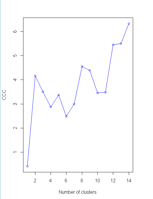
plot(nc$All.index[,4],type="o",ylab="CCC",xlab="Number of clusters",col="blue")