Sampling Matrix

这些天看了一些关于采样矩阵（大概是这么翻译的）的论文，简单做个总结。

• FAST MONTE CARLO ALGORITHMS FOR MATRICES I: APPROXIMATING MATRIX MULTIPLICATION

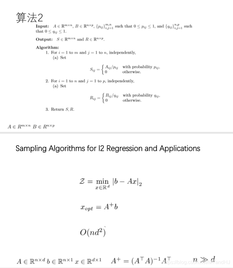
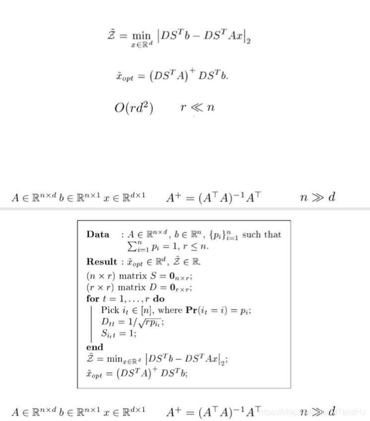
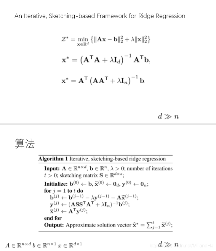
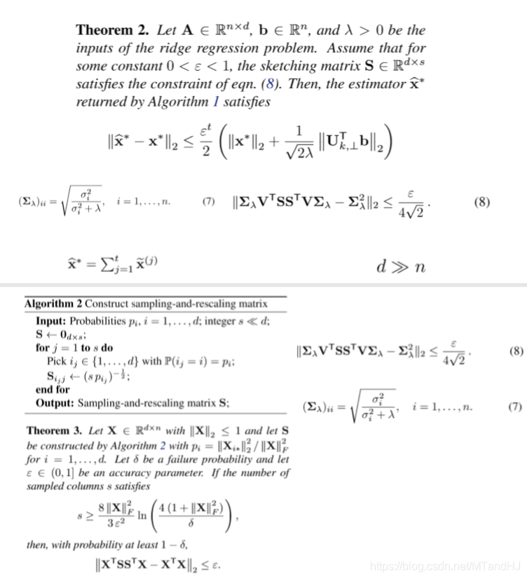
算法如下：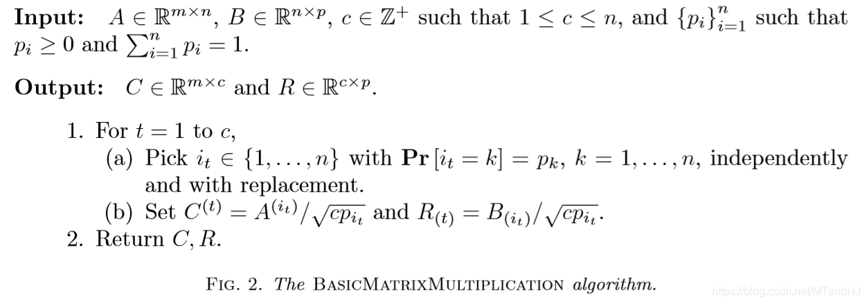

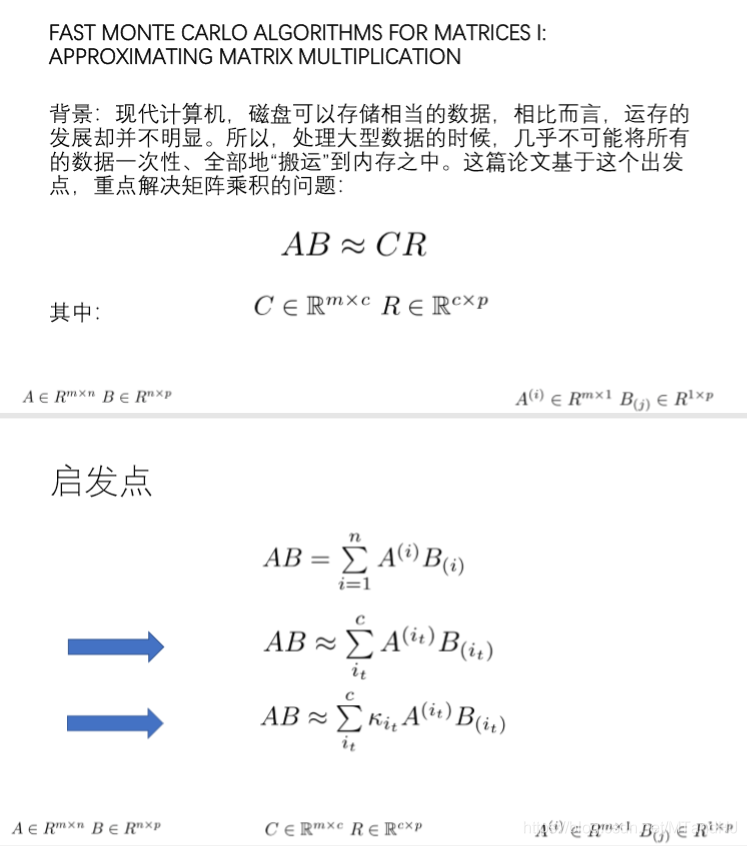
目的是为了毕竟矩阵的乘积AB， 以CR来替代。
其中右上角带有i_t的A表示A的第i_t列，右下角带有i_t的B表示B的第i_t行。

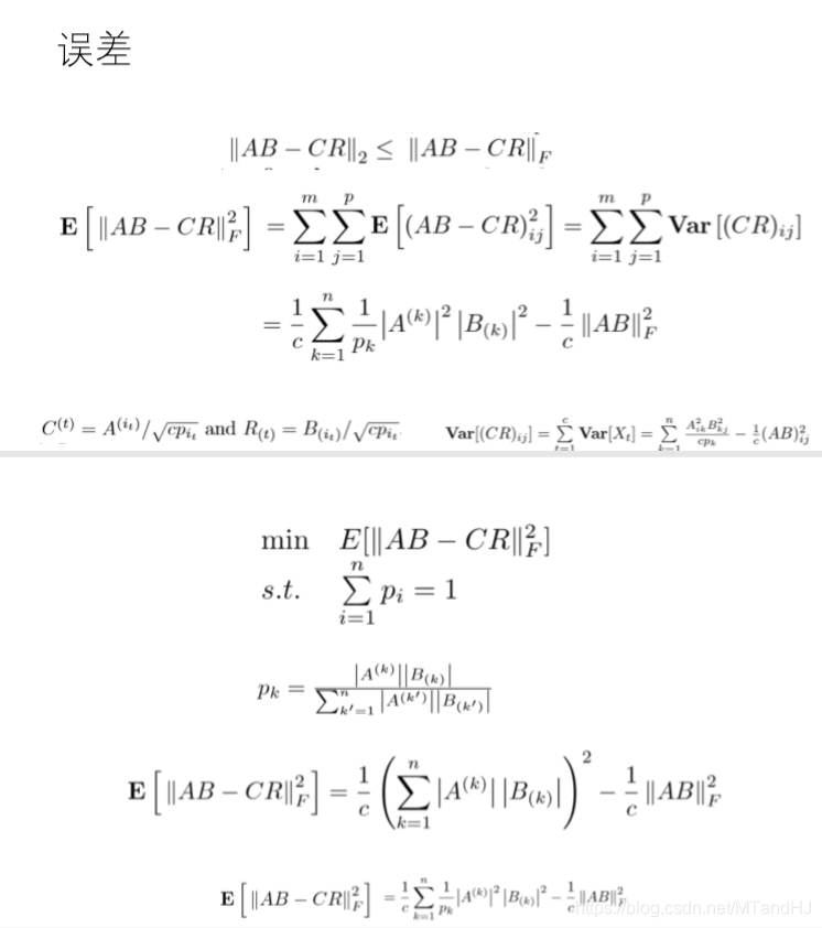
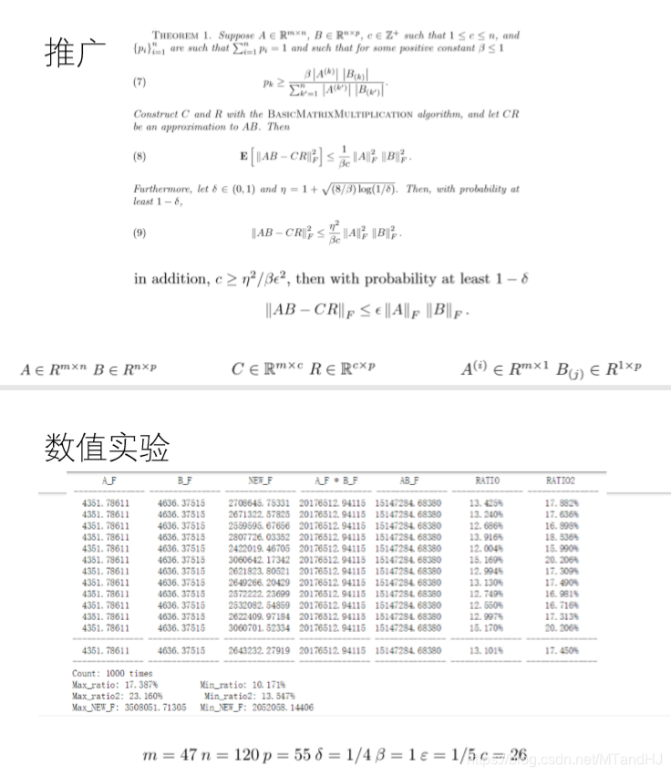
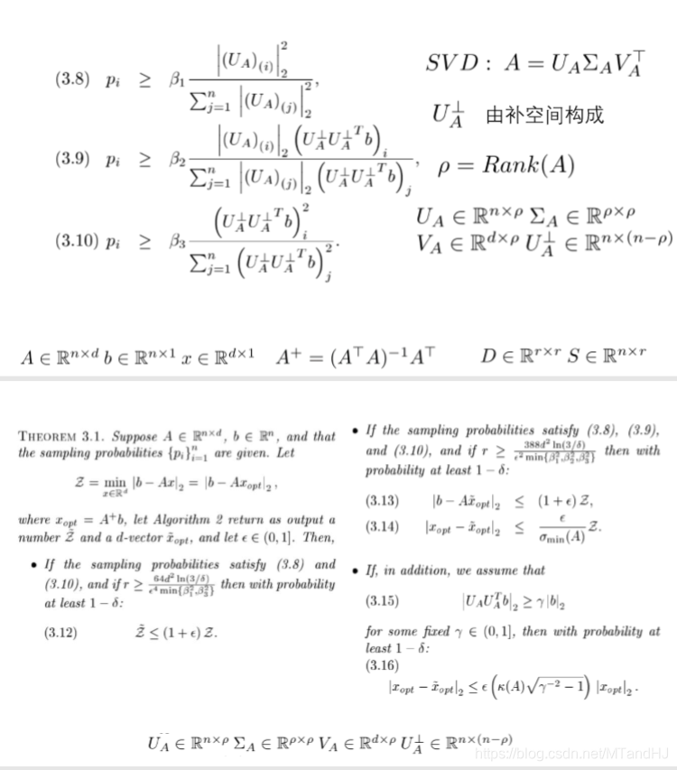
关于 c 的选择，以及误差的估计，请回看论文。
下面是一个小小的测试：
代码：

import numpy as np

def Generate_P(A, B): #生成概率P
    try:
        n1 = len(A[1,:])
        n2 = len(B[:,1])
        if n1 == n2:
            n = n1
        else:
            print('Bad matrices')
            return 0
    except:
        print('The matrices are not fit...')
    A_New = np.square(A)
    B_New = np.square(B)
    P_A = np.array([np.sqrt(np.sum(A_New[:,i])) for i in range(n)])
    P_B = np.array([np.sqrt(np.sum(B_New[i,:])) for i in range(n)])
    P = P_A * P_B / (np.sum(P_A * P_B))
    return P

def Generate_S(n, c, P): #生成采样矩阵S  简化了一下算法
    S = np.zeros((n, c))
    T = np.random.choice(np.array([i for i in range(n)]), size = c, replace = True, p = P)
    for i in range(c):
        S[T[i], i] = 1 / np.sqrt(c * P[T[i]])
    
    return S
    
def Summary(times, n, c, P, A_F, B_F, AB):  #总结和分析
    print('{0:^15} {1:^15} {2:^15} {3:^15} {4:^15} {5:^15} {6:^15}'.format('A_F', 'B_F', 'NEW_F', 'A_F * B_F', 'AB_F', 'RATIO', 'RATIO2'))
    print('{0:-<15} {0:-<15} {0:-<15} {0:-<15} {0:-<15} {0:-<15} {0:-<15}'.format(''))
    A_F_B_F = A_F * B_F
    AB_F = np.sqrt(np.sum(np.square(AB)))
    Max = -1
    Min = 99999999999
    Max2 = -1
    Min2 = 99999999999
    Max_NEW_F = 0
    Min_NEW_F = 0
    Mean_NEW_F = 0
    Mean_ratio = 0
    Mean_ratio2 = 0
    for i in range(times):
        S = Generate_S(n, c, P)
        CR = np.dot(A.dot(S), (S.T).dot(B))
        NEW = AB - CR
        NEW_F = np.sqrt(np.sum(np.square(NEW)))
        ratio = NEW_F / A_F_B_F
        ratio2 = NEW_F / AB_F
        Mean_NEW_F += NEW_F
        Mean_ratio += ratio
        Mean_ratio2 += ratio2
        if ratio > Max:
            Max = ratio
            Max2 = ratio2
            Max_NEW_F = NEW_F
        if ratio < Min:
            Min = ratio
            Min2 = ratio2
            Min_NEW_F = NEW_F
        print('{0:^15.5f} {1:^15.5f} {2:^15.5f} {3:^15.5f} {4:^15.5f} {5:^15.3%} {6:^15.3%}'.format(A_F, B_F, NEW_F, A_F_B_F, AB_F, ratio, ratio2))
    Mean_NEW_F = Mean_NEW_F / times
    Mean_ratio = Mean_ratio / times
    Mean_ratio2 = Mean_ratio2 / times
    print('{0:-<15} {0:-<15} {0:-<15} {0:-<15} {0:-<15} {0:-<15} {0:-<15}'.format(''))
    print('{0:^15.5f} {1:^15.5f} {2:^15.5f} {3:^15.5f} {4:^15.5f} {5:^15.3%} {6:^15.3%}'.format(A_F, B_F, Mean_NEW_F, A_F_B_F, AB_F, Mean_ratio, Mean_ratio2))
    print('{0:-<15} {0:-<15} {0:-<15} {0:-<15} {0:-<15} {0:-<15} {0:-<15}'.format(''))
    print('Count: {0} times'.format(times))
    print('Max_ratio: {0:<15.3%} Min_ratio: {1:<15.3%}'.format(Max, Min))
    print('Max_ratio2: {0:<15.3%} Min_ratio2: {1:<15.3%}'.format(Max2, Min2))
    print('Max_NEW_F: {0:<15.5f} Min_NEW_F: {1:<15.5f}'.format(Max_NEW_F, Min_NEW_F))


#下面是关于矩阵行列的一些参数，我是采用均匀分布产生的矩阵
m = 47
n = 120
p = 55
A = np.array([[np.random.rand() * 100 for j in range(n)] for i in range(m)])
B = np.array([[np.random.rand() * 100 for j in range(p)] for i in range(n)])

#构建c的一些参数 这个得参考论文
Thelta = 1/4
Belta = 1
Yita = 1 + np.sqrt((8/Belta * np.log(1/Thelta)))
e = 1/5
c = int(1 / (Belta * e ** 2)) + 1
P = Generate_P(A, B)

#结果分析
AB = A.dot(B)
A_F = np.sqrt(np.sum(np.square(A)))
B_F = np.sqrt(np.sum(np.square(B)))
times = 1000
Summary(times, n, c, P, A_F, B_F, AB)

   
    

粗略的结果：

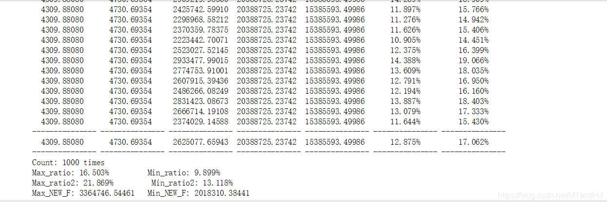
用了原矩阵的一半的维度，代价是约17%的误差。
用正态分布生成矩阵的时候，发现，如果是标准正态分布，效果很差，我猜是由计算机舍入误差引起的，这样的采样的性能不好。当均值增加的时候，和”均匀分布“差不多，甚至更优（F范数的意义上）。

补充：