006-卷积神经网络

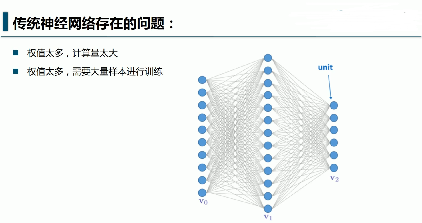
经验之谈：

一般样本的大小是权值的5~10倍

 

import tensorflow as tf
from tensorflow.examples.tutorials.mnist import input_data

mnist = input_data.read_data_sets('MNIST_data/',one_hot= True)

#每个批次的大小：
batch_size = 128

#计算一共有多少批次
n_batch = mnist.train.num_examples//batch_size

#初始化权重值W：
def weight_variable(shape):
    initial = tf.truncated_normal(shape=shape,stddev=0.1)
    return tf.Variable(initial)
#初始化偏置值b
def biases_variable(shape):
    initial = tf.constant(0.1,shape=shape)
    return tf.Variable(initial)

#卷积层
def conv2d(x,W):
    ''' x-input tensor of shape [batch,in_height,in_weight,in_channels]
        W-filter/kernel tensor of shape [filter_height,filter_weight,
                                        in_channels,out_channels]
        stride[0]=stride[3]=1,
        stride[1]-x步长
        stride[2]-y步长
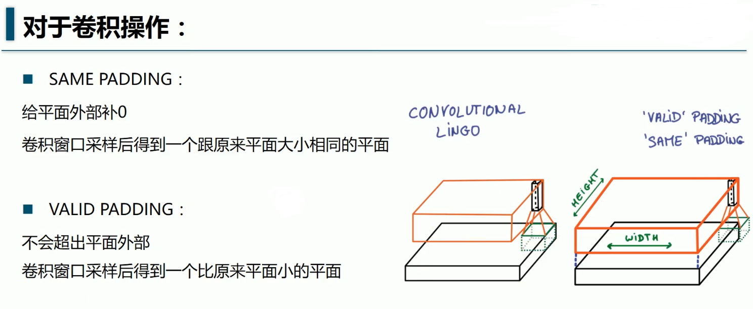
        padding-SAME如果不够则补零(卷积后图像大小与输入一致)，VALID-不补（多余的舍弃）
    '''
    return tf.nn.conv2d(x,W,strides=[1,1,1,1],padding='SAME')

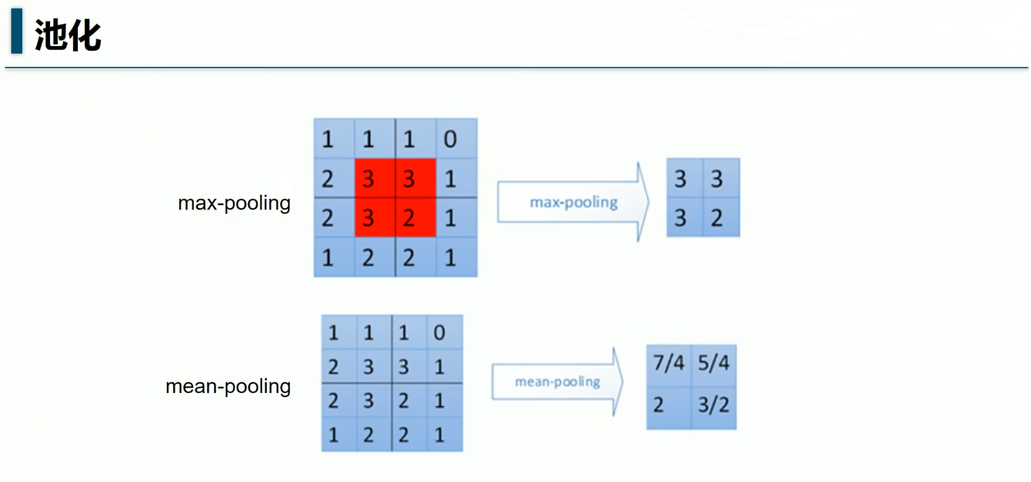
#池化层
def max_pool_2x2(x):
    '''ksize[1,x,y,1],x,y表示窗口大小'''
    return tf.nn.max_pool(x,ksize=[1,2,2,1],strides=[1,2,2,1],padding='SAME')


#定义2个placeholder
x = tf.placeholder(tf.float32,[None,784]) #28x28
y = tf.placeholder(tf.float32,[None,10])

#将x转换为向量
'''[batch,in_height,in_weight,in_channels]'''
x_image = tf.reshape(x,[-1,28,28,1])

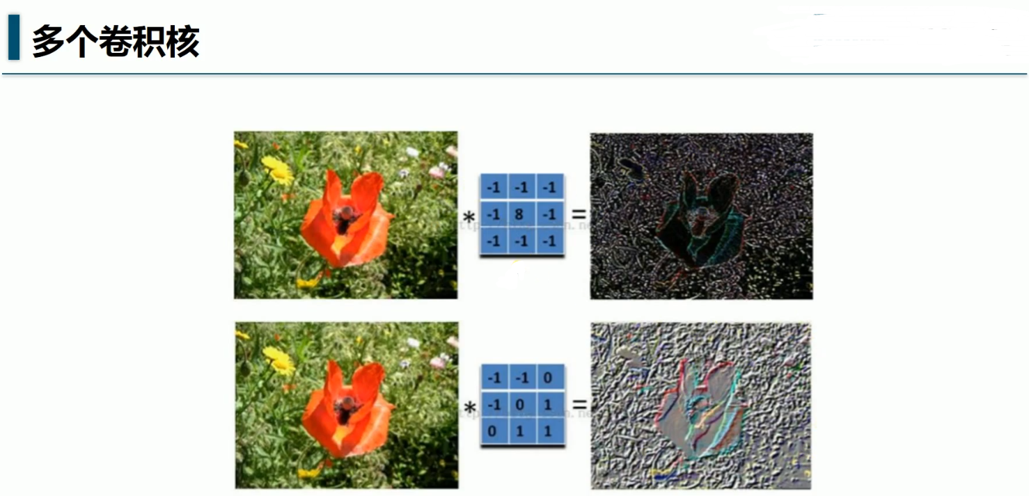
#初始化第一个卷积层的W，b
'''窗口x，窗口y，channels，卷积核filter个数（特征图数量）'''
W_conv1 = weight_variable([5,5,1,32])
'''每一个卷积核对应一个偏置值'''
b_conv1 = biases_variable([32])


#第一层的卷积与池化
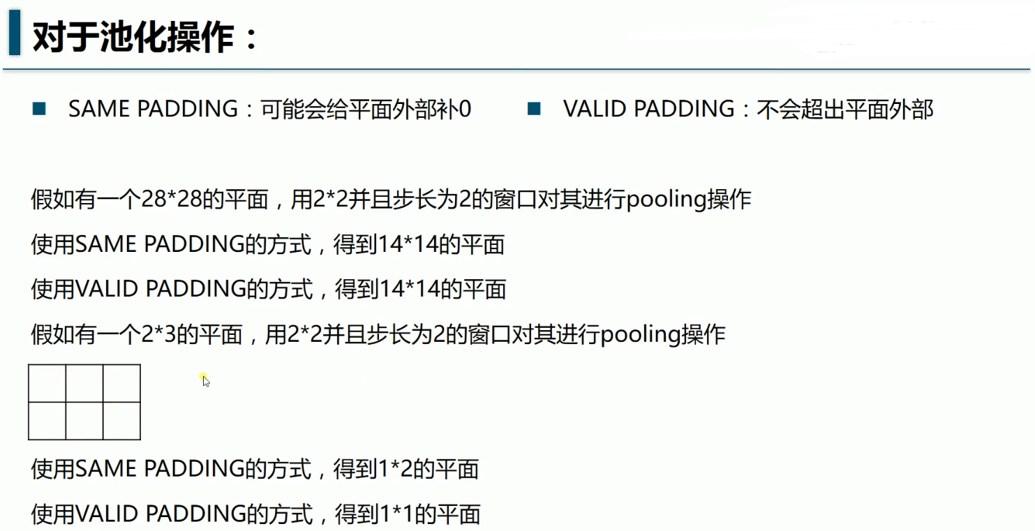
'''28%2=0，所以SAME不补，padding=0，池化后的x应该是，
    （（28+2×0-2）/2 ）+1=14
    第1个2是2倍的padding，第2个2是窗口x=2，第三个2是stride
    池化输入与窗口都是正方形，所以池化后的y=14 ，
    池化后图片14×14
'''
h_conv1 = tf.nn.relu(conv2d(x_image,W_conv1)+b_conv1)
h_pool1 = max_pool_2x2(h_conv1) #14×14，32张


#初始化第二个卷积层的W，b
'''窗口x，窗口y，channels（上一层特征图数量），卷积核filter个数（特征图数量）'''
W_conv2 = weight_variable([5,5,32,64])
'''每一个卷积核对应一个偏置值'''
b_conv2 = biases_variable([64])

#第二层的卷积与池化
'''（（14+2×0-2）/2 ）+1=7，7×7'''
h_conv2 = tf.nn.relu(conv2d(h_pool1,W_conv2)+b_conv2)
h_pool2 = max_pool_2x2(h_conv2)#7×7，64张

#初始化第一个全连接层
W_fc1 = weight_variable([7*7*64,1024])
b_fc1 = biases_variable([1024])

#求第一个全连接层的输出
#1，将最后一层卷积池化层的输出变为扁平化
h_pool2_flat = tf.reshape(h_pool2,[-1,7*7*64])
#2,计算全连接层的输出
h_fc1 = tf.nn.relu(tf.matmul(h_pool2_flat,W_fc1)+b_fc1) #-1×1024

#keep_prob用来表示全连接层的输出率
keep_prob = tf.placeholder(tf.float32)
h_fc1_drop = tf.nn.dropout(h_fc1,keep_prob)

#初始化第二个全连接层
W_fc2 = weight_variable([1024,10])
b_fc2 = biases_variable([10])

#计算输出
'''
-1是batch，这里的batch是100，
所以这里输出的是100×10，
也就是每行是1张图片，一共有100行
每一列是1个特征，一共有10列
'''
prediction = tf.nn.softmax(tf.matmul(h_fc1,W_fc2)+b_fc2) #-1×10



#交叉熵损失函数
coss_entropy = tf.reduce_mean(tf.nn.softmax_cross_entropy_with_logits_v2(labels=y,logits= prediction))                              

#使用Adam优化器
train_step = tf.train.AdamOptimizer(1e-4).minimize(coss_entropy)

#结果存放在一个布尔列表中
correct_prediction = tf.equal(tf.argmax(prediction,1),tf.argmax(y,1))

#求准确率
accuracy = tf.reduce_mean(tf.cast(correct_prediction,tf.float32))

with tf.Session() as sess:
    sess.run(tf.global_variables_initializer())
    for epoch in range(21):
        for batch in range(n_batch):
            batch_xs,batch_ys = mnist.train.next_batch(batch_size)
            sess.run(train_step,feed_dict = {x:batch_xs,y:batch_ys,keep_prob:0.7})
        
        acc = sess.run(accuracy,feed_dict = {x:mnist.test.images,y:mnist.test.labels,keep_prob:1.0})
        
        print("第"+str(epoch)+"次迭代，测试集准确率是"+str(acc))

自己的小笔记本4×i7，GTX960+4G，跑不起来

在阿里云的天池实验室跑，巨慢，21次迭代需要半个小时

结果：

Extracting MNIST_data/train-images-idx3-ubyte.gz

Extracting MNIST_data/train-labels-idx1-ubyte.gz
Extracting MNIST_data/t10k-images-idx3-ubyte.gz
Extracting MNIST_data/t10k-labels-idx1-ubyte.gz

第0次迭代，测试集准确率是0.7688

第1次迭代，测试集准确率是0.7831

第2次迭代，测试集准确率是0.8829

第3次迭代，测试集准确率是0.8883

第4次迭代，测试集准确率是0.889

第5次迭代，测试集准确率是0.8919

第6次迭代，测试集准确率是0.8908

第7次迭代，测试集准确率是0.893

第8次迭代，测试集准确率是0.894

第9次迭代，测试集准确率是0.8949

第10次迭代，测试集准确率是0.8927

第11次迭代，测试集准确率是0.8935

第12次迭代，测试集准确率是0.8948

第13次迭代，测试集准确率是0.9873

第14次迭代，测试集准确率是0.9881

第15次迭代，测试集准确率是0.9864

第16次迭代，测试集准确率是0.9885

第17次迭代，测试集准确率是0.9906

第18次迭代，测试集准确率是0.9876

第19次迭代，测试集准确率是0.9884

第20次迭代，测试集准确率是0.9902

 最后的准确率达到了99.02%