支持向量机算法的Sklearn完整复现

1 scikit_learn里的SVM

scikit-learn里对SVM的算法实现都在包sklearn.svm下，其中SVC类是用来进行分类的任务，SVR是用来进行数值回归任务的。

在计算机中，可以用离散的数值来代替连续的数值进行回归。

以SVC为例，首先选择SVM核函数，由参数kernel指定，其中linear表示本章介绍的线性函数，它只能产生直线形状的分隔超平面；poly表示本章介绍的多项式核函数，可以构造复杂形状的分隔超平面，rbf表示高斯核函数。

不同核函数需要指定不同参数：

• 线性函数只需要指定参数C，它表示对不符合最大间距规则的样本的惩罚力度，即系数R。
• 多项式核函数，除了参数C外，还需要指定degree，表示多项式的阶数。
• 高斯核函数，除了参数C外，还需要指定gamma值，这个值对应高斯核公式中的
  值

def plot_hyperplane(clf, X, y, 
                    h=0.02, 
                    draw_sv=True, 
                    title='hyperplan'):
    # create a mesh to plot in
    x_min, x_max = X[:, 0].min() - 1, X[:, 0].max() + 1
    y_min, y_max = X[:, 1].min() - 1, X[:, 1].max() + 1
    xx, yy = np.meshgrid(np.arange(x_min, x_max, h),
                         np.arange(y_min, y_max, h))

    plt.title(title)
    plt.xlim(xx.min(), xx.max())
    plt.ylim(yy.min(), yy.max())
    plt.xticks(())
    plt.yticks(())

    Z = clf.predict(np.c_[xx.ravel(), yy.ravel()]) # SVM的分割超平面
    # Put the result into a color plot
    Z = Z.reshape(xx.shape)
    plt.contourf(xx, yy, Z, cmap='hot', alpha=0.5)

    markers = ['o', 's', '^']
    colors = ['b', 'r', 'c']
    labels = np.unique(y)
    for label in labels:
        plt.scatter(X[y==label][:, 0], 
                    X[y==label][:, 1], 
                    c=colors[label], 
                    marker=markers[label])
    # 画出支持向量
    if draw_sv:
        sv = clf.support_vectors_
        plt.scatter(sv[:, 0], sv[:, 1], c='y', marker='x')

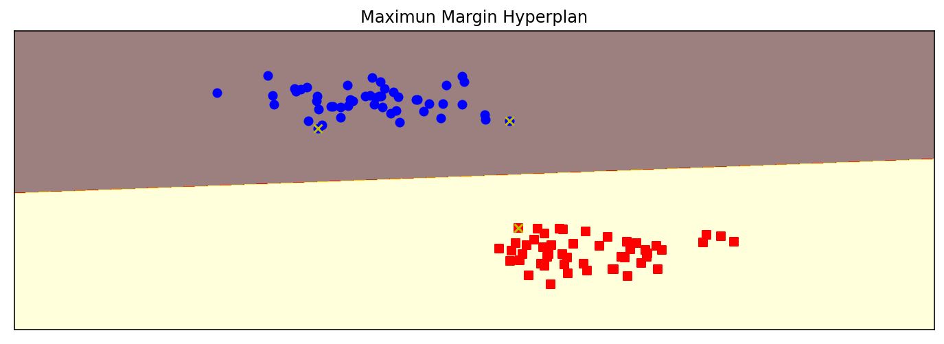
#举一个两特征，两种类的数据集，用SVM对其进行分类
from sklearn import svm
from sklearn.datasets import make_blobs
import matplotlib.pyplot as plt
import numpy as np


X,y = make_blobs(n_samples = 100,centers = 2,random_state = 0,cluster_std = 0.3)
clf = svm.SVC(C = 1.0,kernel = 'linear')
clf.fit(X,y)

plt.figure(figsize = (12,4),dpi = 144)
plot_hyperplane(clf,X,y,h = 0.01,title='Maximun Margin Hyperplan')

​

​

from sklearn import svm
from sklearn.datasets import make_blobs

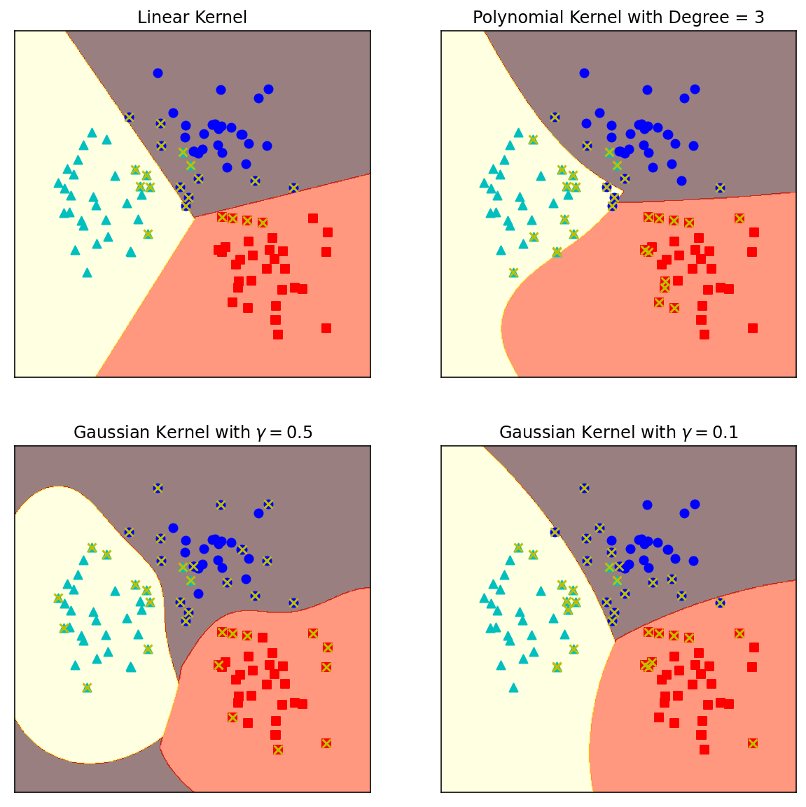
X,y = make_blobs(n_samples = 100,centers = 3,
                    random_state = 0,cluster_std = 0.8)
clf_linear = svm.SVC(C = 1.0,kernel = 'linear')
clf_poly = svm.SVC(C = 1.0,kernel = 'poly',degree = 3)
clf_rbf = svm.SVC(C = 1.0,kernel = 'rbf',gamma = 0.5)
clf_rbf2 = svm.SVC(C = 1.0,kernel = 'rbf',gamma = 0.1)

plt.figure(figsize = (10,10),dpi = 144)

clfs = [clf_linear,clf_poly,clf_rbf,clf_rbf2]
titles = ['Linear Kernel',
         'Polynomial Kernel with Degree = 3',
         'Gaussian Kernel with $gamma = 0.5$',
         'Gaussian Kernel with $gamma = 0.1$']
for clf,i in zip(clfs,range(len(clfs))):
    clf.fit(X,y)
    plt.subplot(2,2,i+1)
    plot_hyperplane(clf,X,y,title = titles[i])

​

​

2. 乳腺癌检测

#载入数据
from sklearn.datasets import load_breast_cancer
from sklearn.model_selection import train_test_split

cancer = load_breast_cancer()
X = cancer.data
y = cancer.target
print('data shape: {0};no.positive; {1};no.negative: {2}'.format(
    X.shape,y[y==1].shape[0],y[y==0].shape[0]))
X_train,X_test,y_train,y_test = train_test_split(X,y,test_size = 0.2)

data shape: (569, 30);no.positive; 357;no.negative: 212

数据集很小，高斯核函数太复杂容易造成过拟合，模型效果应该不会太好。

#运用高斯核函数看模型效果
from sklearn.svm import SVC

clf = SVC(C = 1.0,kernel = 'rbf',gamma = 0.1)
clf.fit(X_train,y_train)
train_score = clf.score(X_train,y_train)
test_score = clf.score(X_test,y_test)
print('train score:{0};test score:{1}'.format(train_score,test_score))

train score:1.0;test score:0.6666666666666666

发现出现了过拟合现象

#使用GridSearchCV来自动选择参数
from common.utils import plot_param_curve
from sklearn.model_selection import GridSearchCV
import numpy as np
import matplotlib.pyplot as plt

gammas = np.linspace(0,0.0003,30)
param_grid = {'gamma':gammas}
clf = GridSearchCV(SVC(),param_grid,cv = 5,return_train_score = True)
clf.fit(X,y)
print("best param:{0}
best score:{1}".format(clf.best_params_,clf.best_score_))
plt.figure(figsize = (10,4),dpi = 144)
plot_param_curve(plt,gammas,clf.cv_results_,xlabel = 'gamma')

best param:{'gamma': 0.00011379310344827585}
best score:0.9367334264865704





<module 'matplotlib.pyplot' from 'D:\Anaconda3\lib\site-packages\matplotlib\pyplot.py'>

​

​

#绘制学习曲线，观察模型拟合情况
import time
from common.utils import plot_learning_curve
from sklearn.model_selection import ShuffleSplit

cv = ShuffleSplit(n_splits = 10,test_size = 0.2,random_state = 0)
title = 'Learning Curves for Gaussian Kernel'

start = time.perf_counter()
plt.figure(figsize = (10,4),dpi = 144)
plot_learning_curve(plt,SVC(C=1.0,kernel = 'rbf',gamma = 0.01),title,X,y,ylim = (0.5,1.01),cv = cv)
print('elaspe:{0:.6f}'.format(time.perf_counter()-start))

elaspe:1.074925

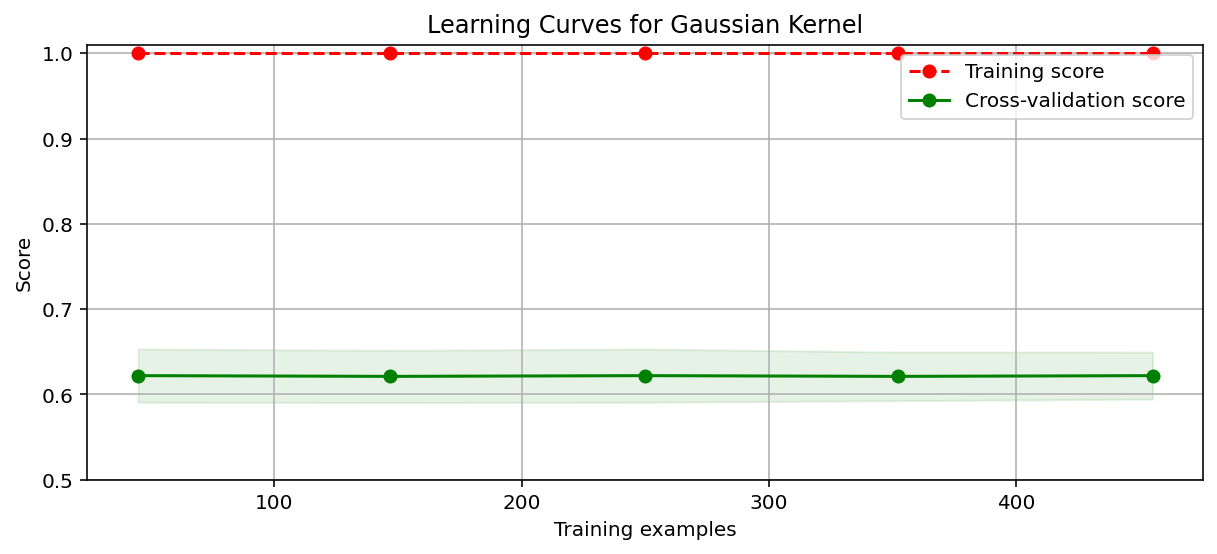
高斯核函数出现明显的过拟合。

#使用二阶多项式核函数进行拟合
from sklearn.svm import SVC

clf = SVC(C = 1.0,kernel = 'poly',degree = 2)
clf.fit(X_train,y_train)
train_score = clf.score(X_train,y_train)
test_score = clf.score(X_test,y_test)
print('train score:{0};test score:{1}'.format(train_score,test_score))

train score:0.9186813186813186;test score:0.9035087719298246

#绘制一阶多项式和二阶多项式学习曲线，观察拟合情况
import time
from common.utils import plot_learning_curve
from sklearn.model_selection import ShuffleSplit

cv = ShuffleSplit(n_splits = 5,test_size = 0.2,random_state = 0)
title = 'Learning Curves with degree = {0}'
degrees = [1,2]

start = time.perf_counter()
plt.figure(figsize = (12,4),dpi = 144)
for i in range(len(degrees)):
    plt.subplot(1,len(degree),i+1)
    plot_learning_curve(plt,SVC(C = 1.0,kernel = 'poly',
                               degree= degrees[i]),
                               title.format(degrees[i]),
                               X,y,ylim = (0.8,1.01),cv = cv,n_jobs = 4)
print('elaspe: {0:.6f}'.format(time.perf_counter()- start))

elaspe: 0.117252