1 好贷款商业前景
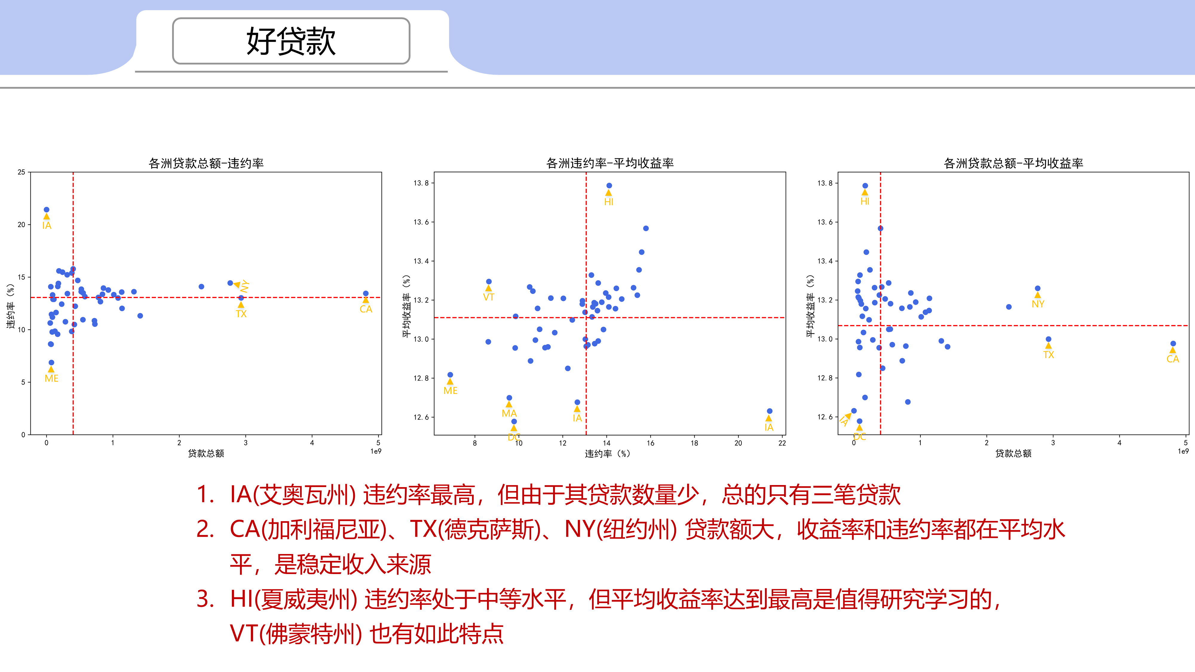
1.1 按地域分析
-
IA(艾奥瓦州) 违约率最高,但由于其贷款数量少,总的只有三笔贷款
-
CA(加利福尼亚)、TX(德克萨斯)、NY(纽约州) 贷款额大,收益率和违约率都在平均水平,是稳定收入来源
-
HI(夏威夷州) 违约率处于中等水平,但平均收益率达到最高是值得研究学习的,VT(佛蒙特州) 也有如此特点
1.2 收入类型与贷款质量
-
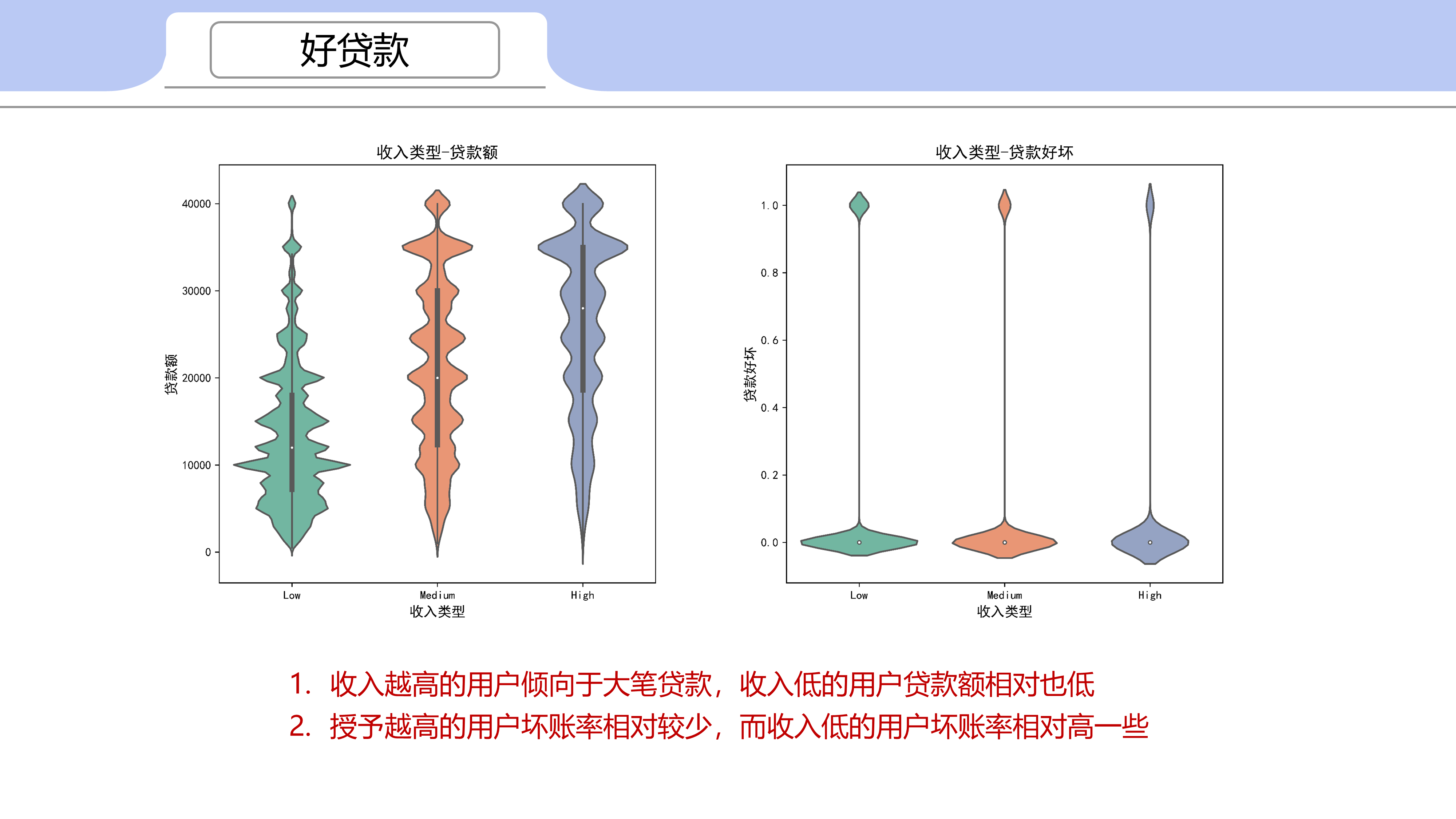
收入越高的用户倾向于大笔贷款,收入低的用户贷款额相对也低
-
收入越高的用户坏账率相对较少,而收入低的用户坏账率相对高一些
2 坏贷款深入查看
2.1 坏款率与住房
-
按揭贷款的用户坏贷款额较高,其次是自有住房用户,最后是租房用户,贷款额逐年增高
2.2 坏款率与贷款利率
-
相对于低利率水平(<13%),高利率水平更容易出现坏账
-
用户在高利率时的长期贷款比 比 低利率时长期贷款比更高
-
相对于长期贷款(60月),短期贷款(36月)更容易出现坏账
2.3 坏款率与贷款等级
-
信用等级良好贷款额逐年上升,信用等级低贷款额在2012年达到顶峰,之后逐年降低
-
贷款利率随着贷款信用等级的降低而提高,信用等级高的用户利率十年间基本维持在统一水平线,而低信用用户则利率逐年上升,甚至达到 30+%
-
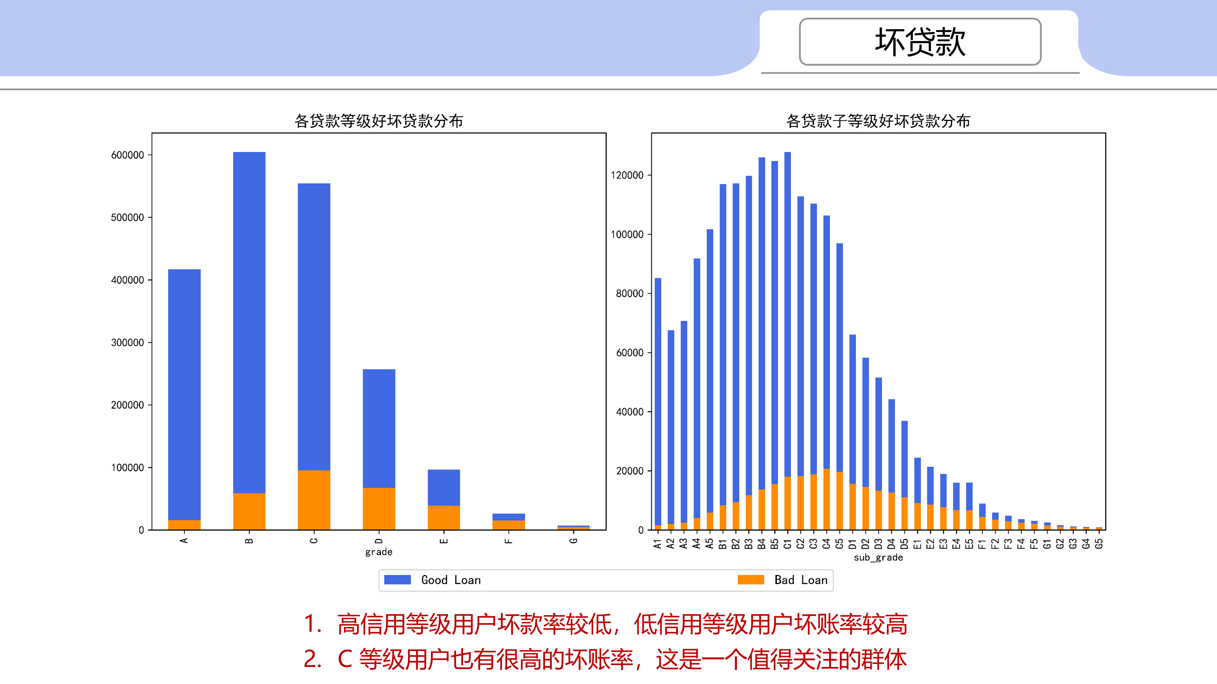
高信用等级用户坏款率较低,低信用等级用户坏账率较高
-
C 等级用户也有很高的坏账率,这是一个值得关注的群体
2.4 坏款率与目的
-
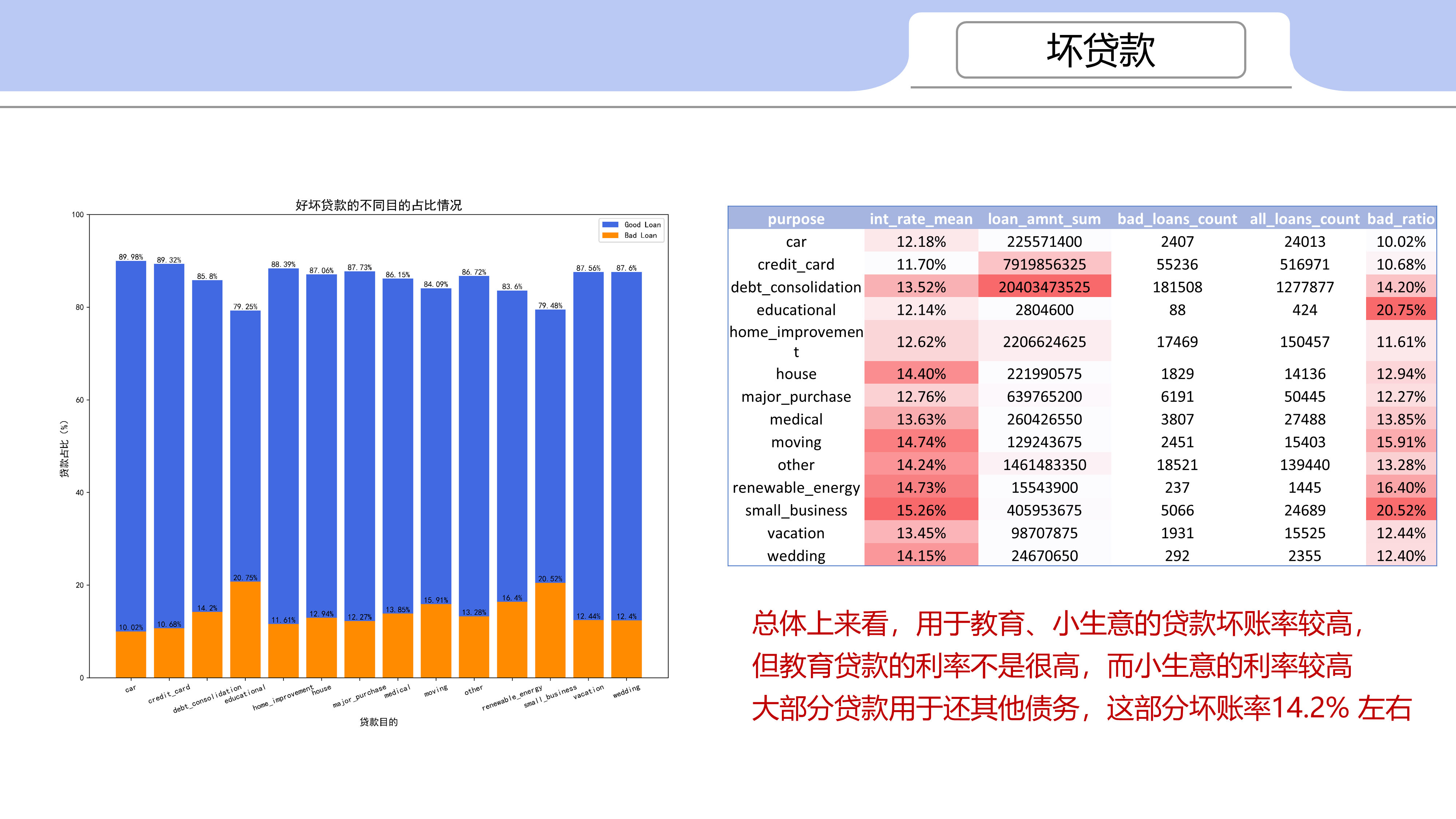
总体上来看,用于教育、小生意的贷款坏账率较高,但教育贷款的利率不是很高,而小生意的利率较高
-
大部分贷款用于还其他债务,这部分坏账率14.2% 左右
-
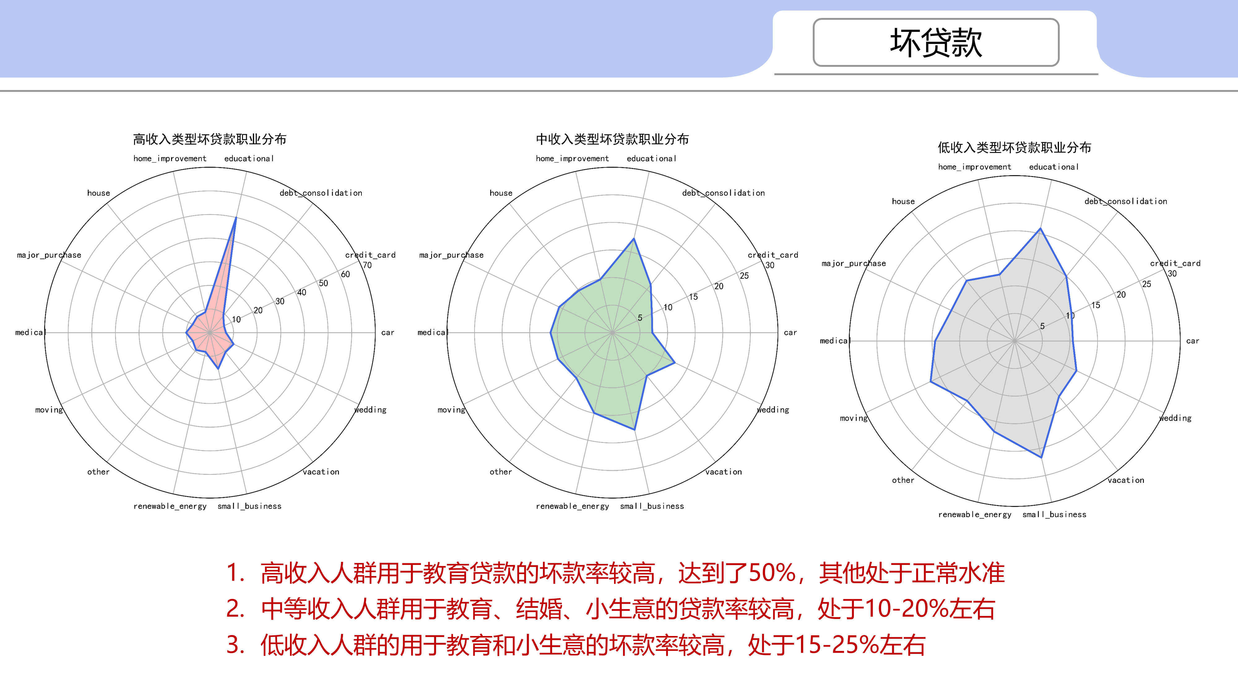
高收入人群用于教育贷款的坏款率较高,达到了50%,其他处于正常水准
-
中等收入人群用于教育、结婚、小生意的贷款率较高,处于10-20%左右
-
低收入人群的用于教育和小生意的坏款率较高,处于15-25%左右


附录代码:
#coding:utf-8
import pandas as pd
import numpy as np
import time
import matplotlib.pyplot as plt
import seaborn as sns
plt.rcParams['font.sans-serif'] = ['SimHei'] # 用来正常显示中文标签
plt.rcParams['axes.unicode_minus'] = False # 用来正常显示负号,#有中文出现的情况,需要u'内容'
# 核心代码,设置显示的最大列、宽等参数,消掉打印不完全中间的省略号
pd.set_option('display.max_columns', 1000)
pd.set_option('display.width', 1000)
pd.set_option('display.max_colwidth', 1000)
start_time = time.process_time()
# # # 读取数据
# loan = pd.read_csv('loan.csv',low_memory = False)
# # df = loan[['issue_d','addr_state','emp_length', 'emp_title', 'annual_inc','home_ownership',
# # 'pub_rec', 'dti','purpose',
# # 'loan_amnt','funded_amnt','funded_amnt_inv','term', 'grade', 'sub_grade','int_rate','loan_status',
# # 'tot_cur_bal','avg_cur_bal', 'total_acc', 'total_bc_limit']].copy()
# df=loan.copy()
# # 将 ‘issue_d’ str形式的时间日期转换
# dt_series = pd.to_datetime(df['issue_d'])
# df['year'] = dt_series.dt.year
# df['month'] = dt_series.dt.month
#
# # 根据收入 'annual_inc' 定义收入“低、中、高”
# # <10万 --> low , 10万~20万 --> medium , >20 万 --> high
# df['income_category'] = np.nan
# lst = [df]
# for col in lst:
# col.loc[col['annual_inc'] <= 100000, 'income_category'] = 'Low'
# col.loc[(col['annual_inc'] > 100000) & (col['annual_inc'] <= 200000), 'income_category'] = 'Medium'
# col.loc[col['annual_inc'] > 200000, 'income_category'] = 'High'
#
# # 根据贷款状态 ‘loan_status’ 定义好坏贷款
# bad_loan = ["Charged Off",
# "Default",
# "Does not meet the credit policy. Status:Charged Off",
# "In Grace Period",
# "Late (16-30 days)",
# "Late (31-120 days)"]
# df['loan_condition'] = np.nan
#
# def loan_condition(status):
# if status in bad_loan:
# return 'Bad Loan'
# else:
# return 'Good Loan'
#
# df['loan_condition'] = df['loan_status'].apply(loan_condition)
# df['loan_condition_int'] = np.nan
# for col in lst:
# col.loc[df['loan_condition'] == 'Good Loan', 'loan_condition_int'] = 0 # Negative (Bad Loan)
# col.loc[df['loan_condition'] == 'Bad Loan', 'loan_condition_int'] = 1 # Positive (Good Loan)
# df['loan_condition_int'] = df['loan_condition_int'].astype(int)
#
# # df.to_pickle("second_df.pkl")
# df.to_pickle("loan_condition.pkl")
#
df = pd.read_pickle('second_df.pkl')
df_state = df.groupby('addr_state').agg({'loan_amnt':'sum','annual_inc':'sum','int_rate':'mean',
'loan_condition_int':'sum','loan_status':'count',
'dti':'mean'}).reset_index()
df_state = df_state.rename(columns = {'loan_amnt':'loan_amnt_sum','annual_inc':'annual_inc_sum','int_rate':'int_rate_mean',
'loan_condition_int':'default_num','loan_status':'loan_num','dti':'dti_mean'})
df_state['default_rate'] = df_state['default_num']/df_state['loan_num']*100
# # 3. 好贷款,有前景
# # 3.1 各个地区 贷款量、违约率、收益率之间关系
# print(df_state.sort_values(by='default_rate'))
# print(df_state.sort_values(by='int_rate_mean'))
# print(df_state.sort_values(by='loan_amnt_sum'))
# print(df_state.sort_values(by='annual_inc_sum'))
# print(df_state.sort_values(by='dti_mean'))
# print(df_state.columns)
#
# fig1_1 = plt.figure(figsize=(6,5))
# ax = fig1_1.add_subplot(111)
# plt.scatter(df_state['default_rate'],df_state['int_rate_mean'],color='royalblue',s=40)
# plt.ylabel('平均收益率(%)',fontsize=12)
# plt.xlabel('违约率(%)',fontsize=12)
# plt.title('各洲违约率-平均收益率',fontsize=16)
# plt.axhline(df_state['int_rate_mean'].mean(),color='r',linestyle='--')
# plt.axvline(df_state['default_rate'].median(),color='r',linestyle='--')
# plt.subplots_adjust(top=1,bottom=0,left=0,right=1,hspace=0,wspace=0)
# plt.savefig("3.1.1 2007-2015 Lending Club 各洲违约率-平均收益率.png",dpi=1000,bbox_inches = 'tight')#解决图片不清晰,不完整的问题
# # plt.show()
#
#
# fig1_2 = plt.figure(figsize=(6,5))
# ax = fig1_2.add_subplot(111)
# plt.scatter(df_state['loan_amnt_sum'],df_state['int_rate_mean'],color='royalblue',s=40)
# # plt.ylim(0,25)
# plt.ylabel('平均收益率(%)',fontsize=12)
# plt.xlabel('贷款总额',fontsize=12)
# plt.title('各洲贷款总额-平均收益率',fontsize=16)
# plt.axhline(df_state['default_rate'].median(),color='r',linestyle='--')
# plt.axvline(df_state['loan_amnt_sum'].median(),color='r',linestyle='--')
# plt.subplots_adjust(top=1,bottom=0,left=0,right=1,hspace=0,wspace=0)
# plt.savefig("3.1.2 2007-2015 Lending Club 各洲贷款总额-平均收益率.png",dpi=1000,bbox_inches = 'tight')#解决图片不清晰,不完整的问题
# # plt.show()
#
# fig1_3 = plt.figure(figsize=(6,5))
# ax = fig1_3.add_subplot(111)
# plt.scatter(df_state['loan_amnt_sum'],df_state['default_rate'],color='royalblue',s=40)
# plt.ylim(0,25)
# plt.ylabel('违约率(%)',fontsize=12)
# plt.xlabel('贷款总额',fontsize=12)
# plt.title('各洲贷款总额-违约率',fontsize=16)
# plt.axvline(df_state['loan_amnt_sum'].median(),color='r',linestyle='--')
# plt.axhline(df_state['default_rate'].median(),color='r',linestyle='--')
# plt.subplots_adjust(top=1,bottom=0,left=0,right=1,hspace=0,wspace=0)
# plt.savefig("3.1.3 2007-2015 Lending Club 各洲贷款总额-违约率.png",dpi=1000,bbox_inches = 'tight')#解决图片不清晰,不完整的问题
#
# # 2. 贷款质量与收入分布
# fig2,ax=plt.subplots(1,2,figsize=(12,5))
# # plt.suptitle('贷款质量和收入分布', fontsize=16)
# sns.violinplot(x='income_category',y='loan_amnt',data=df,ax=ax[0],palette='Set2')
# ax[0].set_ylabel("贷款额",fontsize=12)
# ax[0].set_xlabel("收入类型",fontsize=12)
# ax[0].set_title("收入类型-贷款额",fontsize=14)
# sns.violinplot(x='income_category',y='loan_condition_int',data=df,ax=ax[1],palette='Set2')
# ax[1].set_ylabel("贷款好坏",fontsize=12)
# ax[1].set_xlabel("收入类型",fontsize=12)
# ax[1].set_title("收入类型-贷款好坏",fontsize=14)
# plt.subplots_adjust(top=1,bottom=0,left=0,right=1,hspace=0,wspace=0.3)
# plt.savefig("3.2 2007-2015 Lending Club 贷款质量和收入分布情况.png",dpi=1000,bbox_inches = 'tight')#解决图片不清晰,不完整的问题
# plt.show()
# 4. 风险评估
# 1. 每年不同状态贷款分布
df_status=df.groupby(by=['loan_status','year']).loan_amnt.mean().unstack(-1)
print("
每年不同状态贷款分布
",df_status)
# 2. 违约贷款地域分布 TX > NY > CA
df_default=df[df['loan_status']=='Default']
print("
违约贷款地域分布
",df_default.groupby(by='addr_state').loan_amnt.sum().sort_values())
# 3. 各地区债务比分布情况
print("
各地区债务比分布情况
",df_state.sort_values(by='dti_mean'))
# # 4. 相关原因
# # a) 各变量相关性 协方差热力图
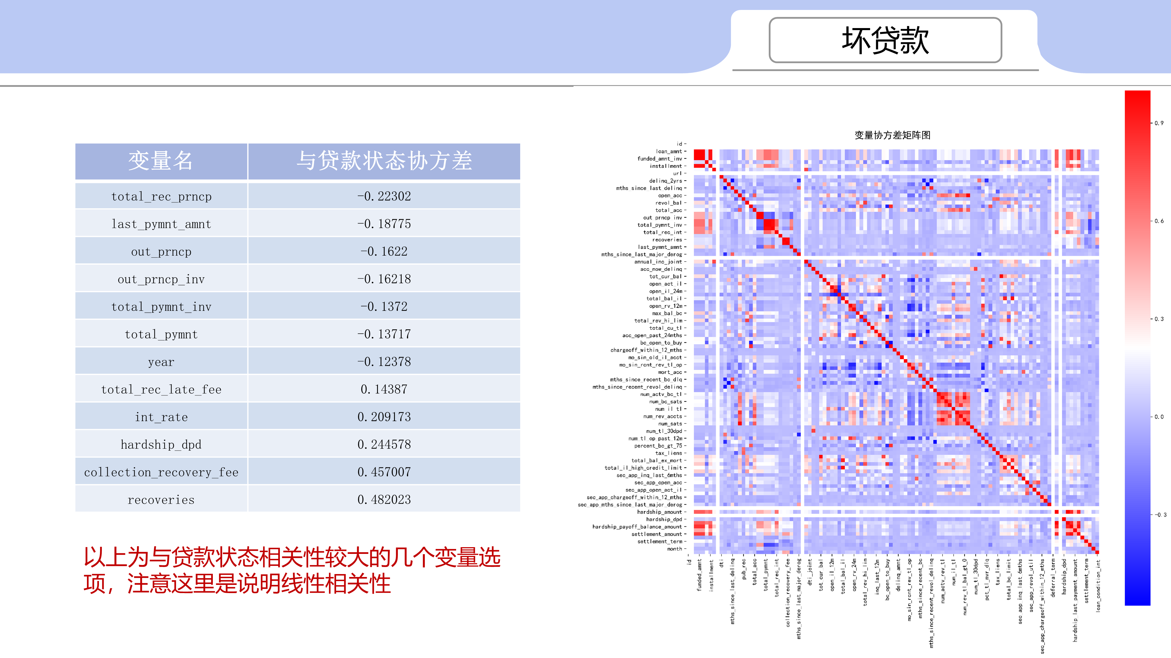
# # 与其从负相关到正相关 分别是 total_rec_prncp ,last_pymnt_amnt ,out_prncp
# # --> total_rec_late_fee,int_rate,hardship_dpd,collection_recovery_fee,recoveries
#
df_all = pd.read_pickle('loan_condition.pkl')
all_corr=df_all.corr()
print("
与坏贷款线性相关性
",all_corr['loan_condition_int'].sort_values())
#
# fig4_1,ax=plt.subplots(figsize=(12,12))
# sns.heatmap(all_corr,cmap='bwr',square=True)
# plt.title('变量协方差矩阵图',fontsize=16)
# plt.subplots_adjust(top=1,bottom=0,left=0,right=1,hspace=0.1,wspace=0.1)
# plt.savefig("4.1 2007-2015 变量协方差矩阵图.png",dpi=1000,bbox_inches = 'tight')#解决图片不清晰,不完整的问题
# # plt.show()
#
# # b) 住房类型-坏贷款
# df_bad=df.loc[df['loan_condition_int']==1]
# fig4_2,ax = plt.subplots(2,1,figsize=(11,5))
#
# sns.boxplot(x='home_ownership',y='loan_amnt',hue='loan_condition',
# data=df_bad,color='royalblue',ax=ax[0])
# ax[0].set_ylabel("贷款额",fontsize=12)
# ax[0].set_xlabel("住房类型",fontsize=12)
# ax[0].set_title("不同住房类型下的坏贷款额分布",fontsize=12)
#
# sns.boxplot(x='year',y='loan_amnt',hue='home_ownership',
# data=df_bad,palette='Set3',ax=ax[1])
# ax[1].set_ylabel("贷款额",fontsize=12)
# ax[1].set_xlabel("年",fontsize=12)
# ax[1].set_title("不同年份不同住房类型下的坏贷款额分布",fontsize=12)
# plt.subplots_adjust(top=1,bottom=0,left=0,right=1,hspace=0.5,wspace=0.1)
# plt.savefig("4.2 2007-2015 不同住房类型与坏贷款额关系.png",dpi=1000,bbox_inches = 'tight')#解决图片不清晰,不完整的问题
# plt.show()
# #
# # c) 收入类型-坏贷款
# df_purpose = df.groupby(by=['income_category','purpose']).aggregate({'int_rate':'mean','loan_amnt':'sum',
# 'loan_condition_int':'sum','loan_condition':'count'}).reset_index()
# df_purpose = df_purpose.rename(columns = {'int_rate':'int_rate_mean','loan_amnt':'loan_amnt_sum',
# 'loan_condition_int':'bad_loans_count','loan_condition':'all_loans_count'})
# df_purpose['bad_ratio'] = df_purpose['bad_loans_count']/df_purpose['all_loans_count']*100
#
# # df_purpose.to_csv('df_purpose.csv')
# df_purpose_high_int = df_purpose[df_purpose['income_category'] == 'High']
# df_purpose_medium_int = df_purpose[df_purpose['income_category'] == 'Medium']
# df_purpose_low_int = df_purpose[df_purpose['income_category'] == 'Low']
#
# # 高中低收入类型的贷款目的分布雷达图
# high_lales = df_purpose_high_int['purpose']
# theta1 = np.linspace(0,2*np.pi,len(high_lales),endpoint = False)
# theta1 = np.concatenate((theta1,[theta1[0]]))
# data1 = df_purpose_high_int['bad_ratio']
# data1 = np.concatenate((data1,[data1[0]]))
#
# fig4_3_1 = plt.figure(figsize=(6,5))
# ax1 = fig4_3_1 .add_subplot(111, polar=True) # polar参数!!
# ax1.plot(theta1, data1, 'royalblue', linewidth=2)# 画线
# ax1.fill(theta1, data1, facecolor='r', alpha=0.25)# 填充
# ax1.set_thetagrids(theta1 * 180/np.pi, high_lales, fontproperties="SimHei")
# ax1.set_title("高收入类型坏贷款职业分布", va='bottom', fontproperties="SimHei",fontsize=14)
# ax1.set_rlim(0,70)
# ax1.grid(True)
# plt.subplots_adjust(top=1,bottom=0,left=0,right=1,hspace=0.1,wspace=0.1)
# plt.savefig("4.3.1 2007-2015 高收入类型坏贷款职业分布.png",dpi=1000,bbox_inches = 'tight') #解决图片不清晰,不完整的问题
# plt.show()
#
# medium_labels = df_purpose_medium_int['purpose']
# theta2 = np.linspace(0,2*np.pi,len(medium_labels),endpoint = False)
# theta2 = np.concatenate((theta2,[theta2[0]]))
# data2 = list(df_purpose_medium_int['bad_ratio'])
# data2 = np.concatenate((data2,[data2[0]]))
#
# fig4_3_2 = plt.figure(figsize=(6,5))
# ax2 = fig4_3_2 .add_subplot(111, polar=True) # polar参数!!
# ax2.plot(theta2, data2, 'royalblue', linewidth=2)# 画线
# ax2.fill(theta2, data2, facecolor='g', alpha=0.25)# 填充
# ax2.set_thetagrids(theta2 * 180/np.pi, medium_labels, fontproperties="SimHei")
# ax2.set_title("中收入类型坏贷款职业分布", va='bottom', fontproperties="SimHei",fontsize=14)
# ax2.set_rlim(0,30)
# ax2.grid(True)
# plt.subplots_adjust(top=1,bottom=0,left=0,right=1,hspace=0.1,wspace=0.1)
# plt.savefig("4.3.2 2007-2015 中收入类型坏贷款职业分布.png",dpi=1000,bbox_inches = 'tight') #解决图片不清晰,不完整的问题
# plt.show()
#
# low_labels = df_purpose_low_int['purpose']
# theta3 = np.linspace(0,2*np.pi,len(low_labels),endpoint = False)
# theta3 = np.concatenate((theta3,[theta3[0]]))
# data3 = list(df_purpose_low_int['bad_ratio'])
# data3 = np.concatenate((data3,[data3[0]]))
#
# fig4_3_3 = plt.figure(figsize=(6,5))
# ax3 = fig4_3_3.add_subplot(111, polar=True) # polar参数!!
# ax3.plot(theta3, data3, 'royalblue', linewidth=2)# 画线
# ax3.fill(theta3, data3, facecolor='grey', alpha=0.25)# 填充
# ax3.set_thetagrids(theta3 * 180/np.pi, low_labels, fontproperties="SimHei")
# ax3.set_title("低收入类型坏贷款职业分布", va='bottom', fontproperties="SimHei",fontsize=14)
# ax3.set_rlim(0,30)
# ax3.grid(True)
# plt.subplots_adjust(top=1,bottom=0,left=0,right=1,hspace=0.1,wspace=0.1)
# plt.savefig("4.3.1 2007-2015 低收入类型坏贷款职业分布.png",dpi=1000,bbox_inches = 'tight') #解决图片不清晰,不完整的问题
# # plt.show()
#
# # d) 贷款利率水平-坏贷款
# # print(df['int_rate'].describe())
# df['int_payments'] = np.nan
# lst = [df]
# for col in lst:
# col.loc[col['int_rate'] <= 13.09, 'int_payments'] = 'Low'
# col.loc[col['int_rate'] > 13.09, 'int_payments'] = 'High'
#
# fig4_4 = plt.figure(figsize=(12,5))
# palette = ['royalblue','darkorange']
# plt.subplot(121)
# ax=sns.countplot(x='int_payments', hue='loan_condition', data = df,palette=palette)
# ax.set_xlabel('利率水平',fontsize=12)
# ax.set_ylabel('贷款额',fontsize=12)
# ax.set_title("不同贷款利率水平下好坏贷款额度情况",fontsize=14)
#
# plt.subplot(122)
# ax1=sns.countplot(x='int_payments', hue='term', data = df,palette=palette)
# ax1.set_xlabel('利率水平',fontsize=12)
# ax1.set_ylabel('贷款额',fontsize=12)
# ax1.set_title("不同贷款利率水平下长短期贷款额度情况",fontsize=14)
# plt.subplots_adjust(top=1,bottom=0,left=0,right=1,hspace=0.1,wspace=0.1)
# plt.savefig("4.4 2007-2015 贷款利率与贷款额关系.png",dpi=1000,bbox_inches = 'tight')#解决图片不清晰,不完整的问题
# # plt.show()
#
#
# # e) 贷款信用等级-坏贷款
# # 每年各个贷款等级贷款额、贷款利率关系
# df_score_loan_amnt = df.groupby(by=['year','grade']).loan_amnt.mean()
# df_score_loan_amnt = df_score_loan_amnt.unstack(-1)
# df_score_int_rate = df.groupby(by=['year','grade']).int_rate.mean()
# df_score_int_rate = df_score_int_rate.unstack(-1)
#
# fig4_5_1,ax = plt.subplots(1,2,figsize=(12,5))
# cmap = plt.cm.coolwarm
# df_score_loan_amnt.plot(legend=False, ax=ax[0], colormap=cmap)
# ax[0].set_title("每年各贷款等级平均发放额",fontsize = 14)
# df_score_int_rate.plot(legend=True, ax=ax[1], colormap=cmap)
# ax[1].legend(bbox_to_anchor=(-1.0, -0.2, 1.7, 0.1), loc=0, prop={'size':12},
# ncol=7, mode="expand", borderaxespad=0.)
# ax[1].set_title("每年各贷款等级平均利率",fontsize = 14)
# plt.subplots_adjust(top=1,bottom=0,left=0,right=1,hspace=0,wspace=0.1)
# plt.savefig("4.5.1 2007-2015 Lending Club 每年贷款等级分布情况.png",dpi=1000,bbox_inches = 'tight')#解决图片不清晰,不完整的问题
# # plt.show()
#
# # 各个贷款等级的贷款好坏分布
# df_score_condition = df.groupby(by=['grade', 'loan_condition']).size()
# df_score_condition = df_score_condition.unstack(-1)
#
# df_score_condition_sub = df.groupby(by=['sub_grade', 'loan_condition']).size()
# df_score_condition_sub = df_score_condition_sub.unstack(-1)
#
# fig4_5_2,ax = plt.subplots(1,2,figsize=(12,5))
# df_score_condition['Good Loan'].plot(kind='bar',legend=False, ax=ax[0], color='royalblue')
# df_score_condition['Bad Loan'].plot(kind='bar',legend=False, ax=ax[0], color='darkorange')
# ax[0].set_title("各贷款等级好坏贷款分布",fontsize = 14)
# df_score_condition_sub['Good Loan'].plot(kind='bar',legend=False, ax=ax[1], color='royalblue')
# df_score_condition_sub['Bad Loan'].plot(kind='bar',legend=False, ax=ax[1], color='darkorange')
# ax[1].set_title("各贷款子等级好坏贷款分布",fontsize = 14)
# ax[1].legend(bbox_to_anchor=(-0.6, -0.2, 1, 0.1), loc=0, prop={'size':12},
# ncol=7, mode="expand", borderaxespad=0.)
# plt.subplots_adjust(top=1,bottom=0,left=0,right=1,hspace=0,wspace=0.1)
# plt.savefig("4.5.2 2007-2015 Lending Club 各贷款等级好坏贷款分布情况.png",dpi=1000,bbox_inches = 'tight')#解决图片不清晰,不完整的问题
# # plt.show()
#
#
# # f) 贷款周期-坏贷款
# fig4_6 = plt.figure(figsize=(6,5))
# palette = ['royalblue','darkorange']
#
# plt.subplot(111)
# ax=sns.countplot(x='term', hue='loan_condition', data = df,palette=palette)
# ax.set_xlabel('贷款周期',fontsize=12)
# ax.set_ylabel('贷款额',fontsize=12)
# ax.set_title("不同贷款周期下好坏贷款额度情况",fontsize=14)
# plt.subplots_adjust(top=1,bottom=0,left=0,right=1,hspace=0,wspace=0.1)
# plt.savefig("4.6 2007-2015 Lending Club 不同贷款周期下好坏贷款额度情况.png",dpi=1000,bbox_inches = 'tight')#解决图片不清晰,不完整的问题
# plt.show()
#
#
# # g) 贷款目的-坏贷款
# # 好坏贷款目的分布直方图
# purpose_condition = round(pd.crosstab(df['loan_condition'], df['purpose']).apply(lambda x: x/x.sum() * 100), 2)
# print()
# ticks=list(purpose_condition.columns)
# x=np.arange(purpose_condition.shape[1])
# y1=purpose_condition.iloc[1,:]
# y2=purpose_condition.iloc[0,:]
#
# fig4_7 = plt.figure(figsize=(10,8))
# p1 = plt.bar(x,y1, color='royalblue')
# p2 = plt.bar(x,y2,color='darkorange')
# for (a,b) in zip(x,y1):
# plt.text(a,b+0.05,s=str(b)+'%',ha='center',va='bottom')
# for (a,b) in zip(x,y2):
# plt.text(a,b+0.05,s=str(b)+'%',ha='center',va='bottom')
# plt.ylim(0,100)
# plt.xticks(x,ticks,rotation=20)
# plt.xlabel('贷款目的',fontsize=12)
# plt.ylabel('贷款占比(%)',fontsize=12)
# plt.title('好坏贷款的不同目的占比情况',fontsize=16)
# plt.legend([p1,p2],labels=['Good Loan','Bad Loan'],loc='best')
# plt.subplots_adjust(top=1,bottom=0,left=0,right=1,hspace=0.1,wspace=0.1)
# plt.savefig("4.7 2007-2015 好坏贷款的不同目的占比情况.png",dpi=1000,bbox_inches = 'tight') #解决图片不清晰,不完整的问题
# plt.show()
#
end_time = time.process_time()
print("程序运行了 %s 秒"%(end_time-start_time))