A brief tour of some of the important components of a Google Datacenter.
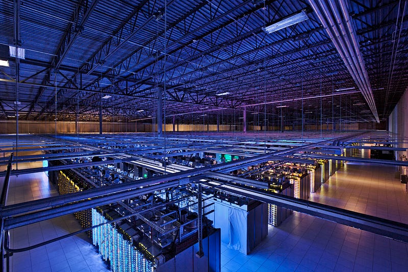
A photo of the interior of a real Google Datacenter in North Carolina. Seen here are rows of racks containing machines.
I am a Site Reliability Engineer at Google, annotating the SRE book in a series of posts. The opinions stated here are my own, not those of my company.
This is Chapter 2: The Production Environment at Google, from the Viewpoint of an SRE.
The Production Environment at Google, from the Viewpoint of an SRE
Written by JC van Winkel
Edited by Betsy Beyer
Google datacenters are very different from most conventional datacenters and small-scale server farms. These differences present both extra problems and opportunities. This chapter discusses the challenges and opportunities that characterize Google datacenters and introduces terminology that is used throughout the book.
Wheeeeeee. We’re going to go on a whirlwind tour of some awesome great big datacenters, and talk about how Google SREs interact with them day to day.
This is both important to those of us who work on this stuff, and totally irrelevant! I say it’s important because this gives a good idea about how to work with and think about extremely large scale systems.
Perhaps the relevancy of this chapter is more about setting the context for the rest of the book, rather than providing an exemplar that my readers should strive to emulate, because the number of organisations that run their own planet scale on-premises computing systems is vanishingly small.
I would expect anyone these days who is doing large scale computing to use a cloud service provided by someone such as Amazon, Google or Microsoft.
Hardware
Most of Google’s compute resources are in Google-designed datacenters with proprietary power distribution, cooling, networking, and compute hardware (see [Bar13]). Unlike “standard” colocation datacenters, the compute hardware in a Google-designed datacenter is the same across the board. To eliminate the confusion between server hardware and server software, we use the following terminology throughout the book:
Machine: A piece of hardware (or perhaps a VM)
Server: A piece of software that implements a service
Machines can run any server, so we don’t dedicate specific machines to specific server programs. There’s no specific machine that runs our mail server, for example. Instead, resource allocation is handled by our cluster operating system, Borg.
This is the first point in the book where we make a reference to the policy of keeping ‘Cattle’ not ‘Pets’. This is an important idea: that in order to have a reliable system, you need to make it out of interchangeable and replaceable parts that can fail at any time.
Any of our machines (or indeed: rocks or rows!) can be turned off at any time, and the abstraction layer (Borg) will make sure that the servers that need to keep running are started on suitable machines nearly-immediately.
We realize this use of the word server is unusual. The common use of the word conflates “binary that accepts network connection” with machine, but differentiating between the two is important when talking about computing at Google. Once you get used to our usage of server, it becomes more apparent why it makes sense to use this specialized terminology, not just within Google but also in the rest of this book.
Figure 2–1 illustrates the topology of a Google datacenter:
Tens of machines are placed in a rack.
Fun fact! A ‘Rack’ at Google actually refers to the set of machines connected to a Top-of-Rack switch. So 2 ‘Racks’ according to the cluster management software are actually sometimes in 3 physical racks, because the important failure domain is the switch.
Racks stand in a row.
Each row is a failure domain because they’re connected to the same power.
One or more rows form a cluster.
Always more than one row. Otherwise we can’t do power maintenance!
Usually a datacenter building houses multiple clusters.
Typically 3 clusters per building, sometimes 4. Often clusters in the same building share a network failure domain.
Multiple datacenter buildings that are located close together form a campus.
A campus doesn’t share the same network failure domain, typically there are multiple independent network interconnects to the facility. The failure domain they share is grid power and weather.

Machines within a given datacenter need to be able to talk with each other, so we created a very fast virtual switch with tens of thousands of ports. We accomplished this by connecting hundreds of Google-built switches in a Clos network fabric [Clos53] named Jupiter [Sin15]. In its largest configuration, Jupiter supports 1.3 Pbps bisection bandwidth among servers.
1.3 Pbps bisection bandwidth is so mindbogglingly fast that Google engineers treat inter-machine bandwidth in the same cluster as effectively infinite.
Jupiter is also so fast and so large that each building (see above) connects all machines in 3 clusters to the same Jupiter fabric. This means that every machine in 3 clusters can talk to any other machine at speeds that are effectively only limited by the NICs on the machines themselves.
Datacenters are connected to each other with our globe-spanning backbone network B4 [Jai13]. B4 is a software-defined networking architecture (and uses the OpenFlow open-standard communications protocol). It supplies massive bandwidth to a modest number of sites, and uses elastic bandwidth allocation to maximize average bandwidth [Kum15].
B4 is important to Google because it frequently has to send extremely large amounts of data around the world, such as Search Indexes, Analytics Hits or Ad Impressions. This has to be done at high bandwidth, and economically.
Using high end backbone grade transmission equipment for this would be extremely expensive, so Google has designed and built its own network equipment that met its requirements for high bandwidth bulk data transmissions.
The two technologies, Jupiter and B4, in combination mean that a Google engineer can run an extremely large, network intensive cluster computation in on location, and then transmit the results to Google datacenters all around the world.
System Software That “Organizes” the Hardware
Our hardware must be controlled and administered by software that can handle massive scale. Hardware failures are one notable problem that we manage with software. Given the large number of hardware components in a cluster, hardware failures occur quite frequently. In a single cluster in a typical year, thousands of machines fail and thousands of hard disks break; when multiplied by the number of clusters we operate globally, these numbers become somewhat breathtaking. Therefore, we want to abstract such problems away from users, and the teams running our services similarly don’t want to be bothered by hardware failures. Each datacenter campus has teams dedicated to maintaining the hardware and datacenter infrastructure.
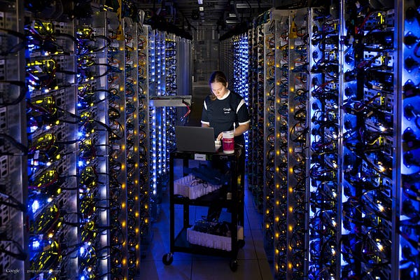
A hardware operations tech replacing components in a failed machine.
Working through the numbers, the MTBF (Mean Time Before Failure) of a machine might be something like 3 years. So if you run a computation that takes 1000 computers just over 1 day to complete, then that’s like running 1 machine for 3 years.
So on average. Every time you run that task, a machine dies. At that scale, you really can’t afford to bothered by machine failures! You might run this once a day, or once a week.
To a Google engineer, 1000 machines is not an unreasonable number of machines to use for their work. For computations like building the search index or for Google Brain we use many more than that, continuously.
Managing Machines
Borg, illustrated in Figure 2–2, is a distributed cluster operating system [Ver15], similar to Apache Mesos. Borg manages its jobs at the cluster level.
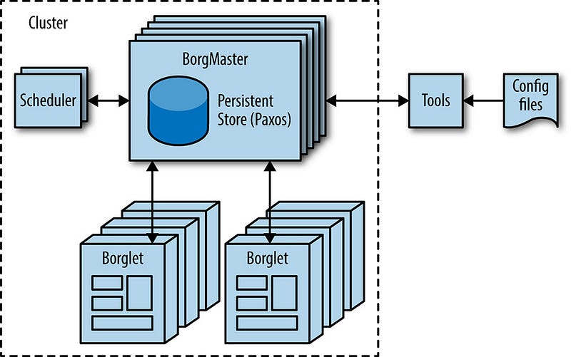
Borg is responsible for running users’ jobs, which can either be indefinitely running servers or batch processes like a MapReduce [Dea04]. Jobs can consist of more than one (and sometimes thousands) of identical tasks, both for reasons of reliability and because a single process can’t usually handle all cluster traffic. When Borg starts a job, it finds machines for the tasks and tells the machines to start the server program. Borg then continually monitors these tasks. If a task malfunctions, it is killed and restarted, possibly on a different machine.
I find it interesting that the book talks about Mesos, but not about Kubernetes. Kubernetes is a cluster management system heavily influenced by the design of Borg.
Because tasks are fluidly allocated over machines, we can’t simply rely on IP addresses and port numbers to refer to the tasks. We solve this problem with an extra level of indirection: when starting a job, Borg allocates a name and index number to each task using the Borg Naming Service (BNS). Rather than using the IP address and port number, other processes connect to Borg tasks via the BNS name, which is translated to an IP address and port number by BNS. For example, the BNS path might be a string such as/bns/<cluster>/<user>/<job name>/<task number>, which would resolve to<IP address>:<port>.
An astute reader might ask, “Why not use SRV records?” or “Why not use IPv6 and have a stable port for the server?”
The primary reason for not using DNS directly is that BNS is implemented using a lockserver, so that everyone who is interested in the addresses of servers can get an update immediately, without waiting for a TTL to expire, or having extremely short TTLs. The lockserver we use, called chubby, is referred to later in this chapter. I will rant about it in the next post.
Borg is also responsible for the allocation of resources to jobs. Every job needs to specify its required resources (e.g., 3 CPU cores, 2 GiB of RAM). Using the list of requirements for all jobs, Borg can binpack the tasks over the machines in an optimal way that also accounts for failure domains (for example: Borg won’t run all of a job’s tasks on the same rack, as doing so means that the top of rack switch is a single point of failure for that job).
If a task tries to use more resources than it requested, Borg kills the task and restarts it (as a slowly crashlooping task is usually preferable to a task that hasn’t been restarted at all).
Here is an example of where an SRE (or other astute engineer, lets not limit this to just people with that job title!) might say, “But if job needs more resources than has been asked for, why doesn’t some computer program notice that and increase the resources and make the whole system heal itself?”
The answer is that those systems do exist at Google, and we use them in some places and not others. For instance batch processes nearly always are auto-tuned to have the exact amount they need.
With latency sensitive Internet-serving jobs, suddenly using 2x as much RAM with the latest release is probably a performance regression, and you want to roll back the server as opposed to doubling the usage across the fleet.
Storage
Tasks can use the local disk on machines as a scratch pad, but we have several cluster storage options for permanent storage (and even scratch space will eventually move to the cluster storage model). These are comparable to Lustre and the Hadoop Distributed File System (HDFS), which are both open source cluster filesystems.
The storage layer is responsible for offering users easy and reliable access to the storage available for a cluster. As shown in Figure 2–3, storage has many layers:
The lowest layer is called D (for disk, although D uses both spinning disks and flash storage). D is a fileserver running on almost all machines in a cluster. However, users who want to access their data don’t want to have to remember which machine is storing their data, which is where the next layer comes into play.
D is more of a block server than a file server. It provides nothing apart from checksums.
Google runs D on practically all machines, and there’s an expectation that you will access data via D rather than using local disk for anything.
Because disks are slow, for both seek time and throughput, reading data out of D off many machine simultaneously is can be much faster than reading from local disk. So we devote nearly all disk I/O time to D!
A layer on top of D called Colossus creates a cluster-wide filesystem that offers usual filesystem semantics, as well as replication and encryption. Colossus is the successor to GFS, the Google File System [Ghe03].
GFS didn’t scale very well, and its fault tolerance left a lot to be desired. It was being actively decommissioned when I joined Google in 2011, and is now totally dead. The code has been deleted.
Colossus is a rock solid scalable storage system, especially in comparison to GFS.
There are several database-like services built on top of Colossus:
Bigtable [Cha06] is a NoSQL database system that can handle databases that are petabytes in size. A Bigtable is a sparse, distributed, persistent multidimensional sorted map that is indexed by row key, column key, and timestamp; each value in the map is an uninterpreted array of bytes. Bigtable supports eventually consistent, cross-datacenter replication.
Bigtable is described as “NoSQL” here, but is from years before NoSQL was a term commonly used. It sits apart somewhat because its interface is somewhat different to someone used to NoSQL meaning a way of storing JSON blobs.
Bigtable is really quite hard to use unless you’re doing something bigtable is really good at.
For instance: Bigtable is really good at being an ordered key-value storage system for terabytes to petabytes of data. Especially if you want to subsequently apply some function (i.e. a MapReduce) to all that data as fast as possible.
Bigtable is not a great database if you want consistency across multiple datacenters, which is a design constraint that most systems at Google that want to store data on behalf of customers have.
Spanner [Cor12] offers an SQL-like interface for users that require real consistency across the world.
You may have heard that Google released Google Cloud Spanner, so that Google Cloud customers can use it.
Spanner is a planet scale database that uses time-travel to provide strong consistency faster than the speed of light would ordinarily allow. It was invented by Jeff Dean, who is one of Google’s brightest stars.
Jeff has a certain mystique at Google, the same sort of level of respect given to heroes such as Chuck Norris, Batman, or Mr Rogers. My favorite (true!) fact about Jeff Dean is that when he gave a seminar at Stanford, it was so crowded that Donald Knuth had to sit on the floor.
Several other database systems, such as Blobstore, are available. Each of these options comes with its own set of trade-offs (see Data Integrity: What You Read Is What You Wrote).
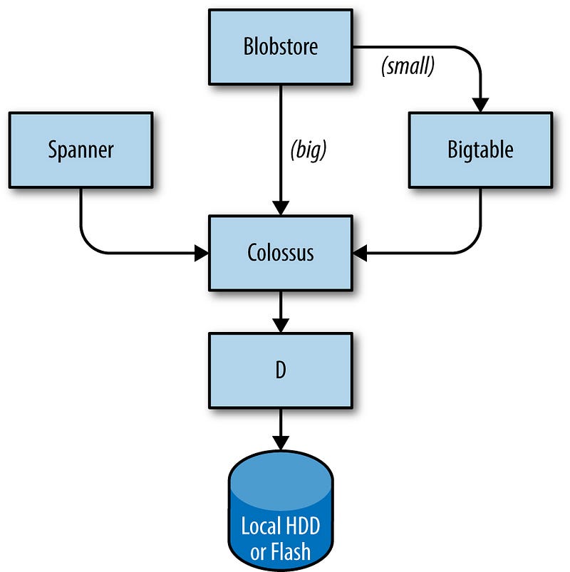
I hope this diagram is understandable. I would perhaps put the ‘Storage’ box labelled ‘Local HDD or Flash’ inside the D box, because they’re intricately linked (if one D server goes away, so does its storage!).
This does make it clear that only D actually stores things.
You might ask: But how does anything know anything about itself if everything’s in D, how do you start and know where your data is in D?
The answer is that a small amount of information (logical equivalent of the ext2 superblock or the FAT table) is stored in chubby. Chubby will be covered in detail in the next post.
原文链接:https://medium.com/@jerub/the-production-environment-at-google-8a1aaece3767