初始化
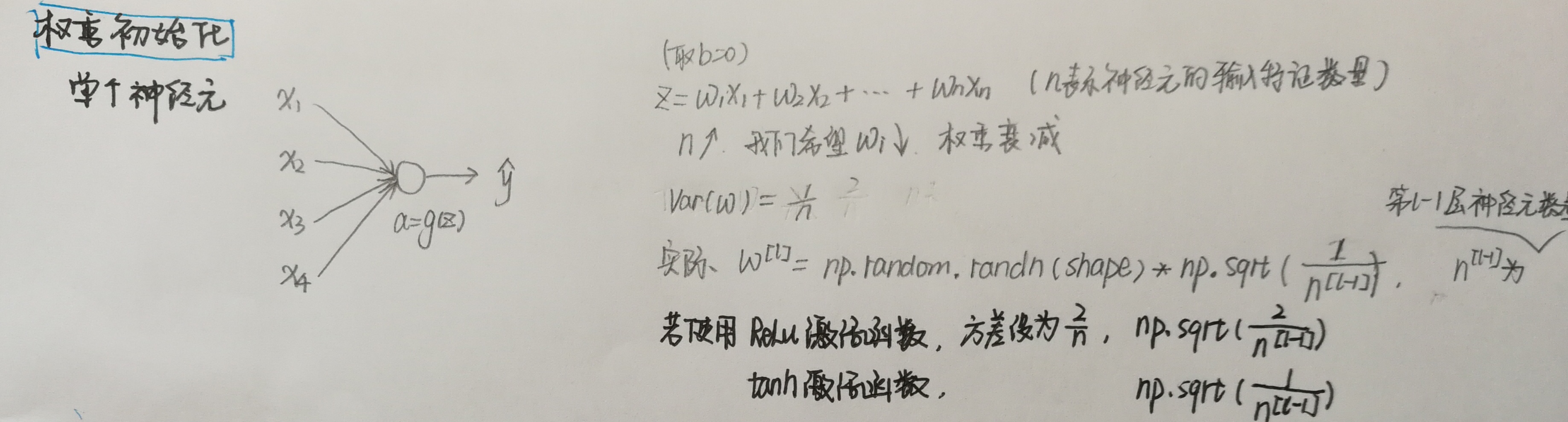
分别使用0、随机数和抑梯度异常初始化参数,比较发现抑梯度异常初始化参数可以得到更高的准确度。
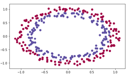
原始数据:
import numpy as np
import matplotlib.pyplot as plt
import sklearn
import sklearn.datasets
from init_utils import sigmoid, relu, compute_loss, forward_propagation, backward_propagation
from init_utils import update_parameters, predict, load_dataset, plot_decision_boundary, predict_dec
from math import sqrt

# %matplotlib inline
plt.rcParams['figure.figsize'] = (7.0, 4.0) # set default size of plots
plt.rcParams['image.interpolation'] = 'nearest'
plt.rcParams['image.cmap'] = 'gray'

# load image dataset: blue/red dots in circles
train_X, train_Y, test_X, test_Y = load_dataset()
使用抑梯度异常初始化代码如下:


  1 #three layers
  2 def model(X, Y, learning_rate=0.01, num_iterations=15000, print_cost=True, initialization="he"):
  3     """
  4     Implements a three-layer neural network: LINEAR->RELU->LINEAR->RELU->LINEAR->SIGMOID.
  5
  6     Arguments:
  7     X -- input data, of shape (2, number of examples)
  8     Y -- true "label" vector (containing 0 for red dots; 1 for blue dots), of shape (1, number of examples)
  9     learning_rate -- learning rate for gradient descent
 10     num_iterations -- number of iterations to run gradient descent
 11     print_cost -- if True, print the cost every 1000 iterations
 12     initialization -- flag to choose which initialization to use ("zeros","random" or "he")
 13
 14     Returns:
 15     parameters -- parameters learnt by the model
 16     """
 17
 18     grads = {}
 19     costs = []     # to keep track of the loss
 20     m = X.shape[1] # number of examples
 21     layers_dims = [X.shape[0], 10, 5, 1]
 22
 23     # Initialize parameters dictionary.
 24     parameters = initialize_parameters_he(layers_dims)
 25
 26     # Loop (gradient descent)
 27     for i in range(0, num_iterations):
 28
 29         # Forward propagation: LINEAR -> RELU -> LINEAR -> RELU -> LINEAR -> SIGMOID.
 30         a3, cache = forward_propagation(X, parameters)
 31
 32         # Loss
 33         cost = compute_loss(a3, Y)
 34
 35         # Backward propagation.
 36         grads = backward_propagation(X, Y, cache)
 37
 38         # Update parameters.
 39         parameters = update_parameters(parameters, grads, learning_rate)
 40
 41         # Print the loss every 1000 iterations
 42         if print_cost and i % 1000 == 0:
 43             print("Cost after iteration {}: {}".format(i, cost))
 44             costs.append(cost)
 45
 46     # plot the loss
 47     plt.plot(costs)
 48     plt.ylabel('cost')
 49     plt.xlabel('iterations (per hundreds)')
 50     plt.title("Learning rate =" + str(learning_rate))
 51     plt.show()
 52
 53     return parameters
 54
 55
 56 # GRADED FUNCTION: initialize_parameters_he
 57 def initialize_parameters_he(layers_dims):
 58     """
 59     Arguments:
 60     layer_dims -- python array (list) containing the size of each layer.
 61
 62     Returns:
 63     parameters -- python dictionary containing your parameters "W1", "b1", ..., "WL", "bL":
 64                     W1 -- weight matrix of shape (layers_dims[1], layers_dims[0])
 65                     b1 -- bias vector of shape (layers_dims[1], 1)
 66                     ...
 67                     WL -- weight matrix of shape (layers_dims[L], layers_dims[L-1])
 68                     bL -- bias vector of shape (layers_dims[L], 1)
 69     """
 70
 71     np.random.seed(3)
 72     parameters = {}
 73     L = len(layers_dims) - 1 # integer representing the number of layers
 74
 75     for l in range(1, L + 1):
 76         ### START CODE HERE ### (≈ 2 lines of code)
 77         parameters['W'+str(l)]=np.random.randn(layers_dims[l], layers_dims[l-1])*sqrt(2./layers_dims[l-1])
 78         parameters['b'+str(l)]=np.zeros((layers_dims[l], 1))
 79         ### END CODE HERE ###
 80     return parameters
 81
 82 parameters = initialize_parameters_he([2, 4, 1])
 83 print("W1 = " + str(parameters["W1"]))
 84 print("b1 = " + str(parameters["b1"]))
 85 print("W2 = " + str(parameters["W2"]))
 86 print("b2 = " + str(parameters["b2"]))
 87
 88
 89 parameters = model(train_X, train_Y, initialization = "he")
 90 print("On the train set:")
 91 predictions_train = predict(train_X, train_Y, parameters)
 92 print("On the test set:")
 93 predictions_test = predict(test_X, test_Y, parameters)
 94
 95
 96 plt.title("Model with He initialization")
 97 axes = plt.gca()
 98 axes.set_xlim([-1.5, 1.5])
 99 axes.set_ylim([-1.5, 1.5])
100 plot_decision_boundary(lambda x: predict_dec(parameters, x.T), train_X, train_Y)
预测准确度0.96

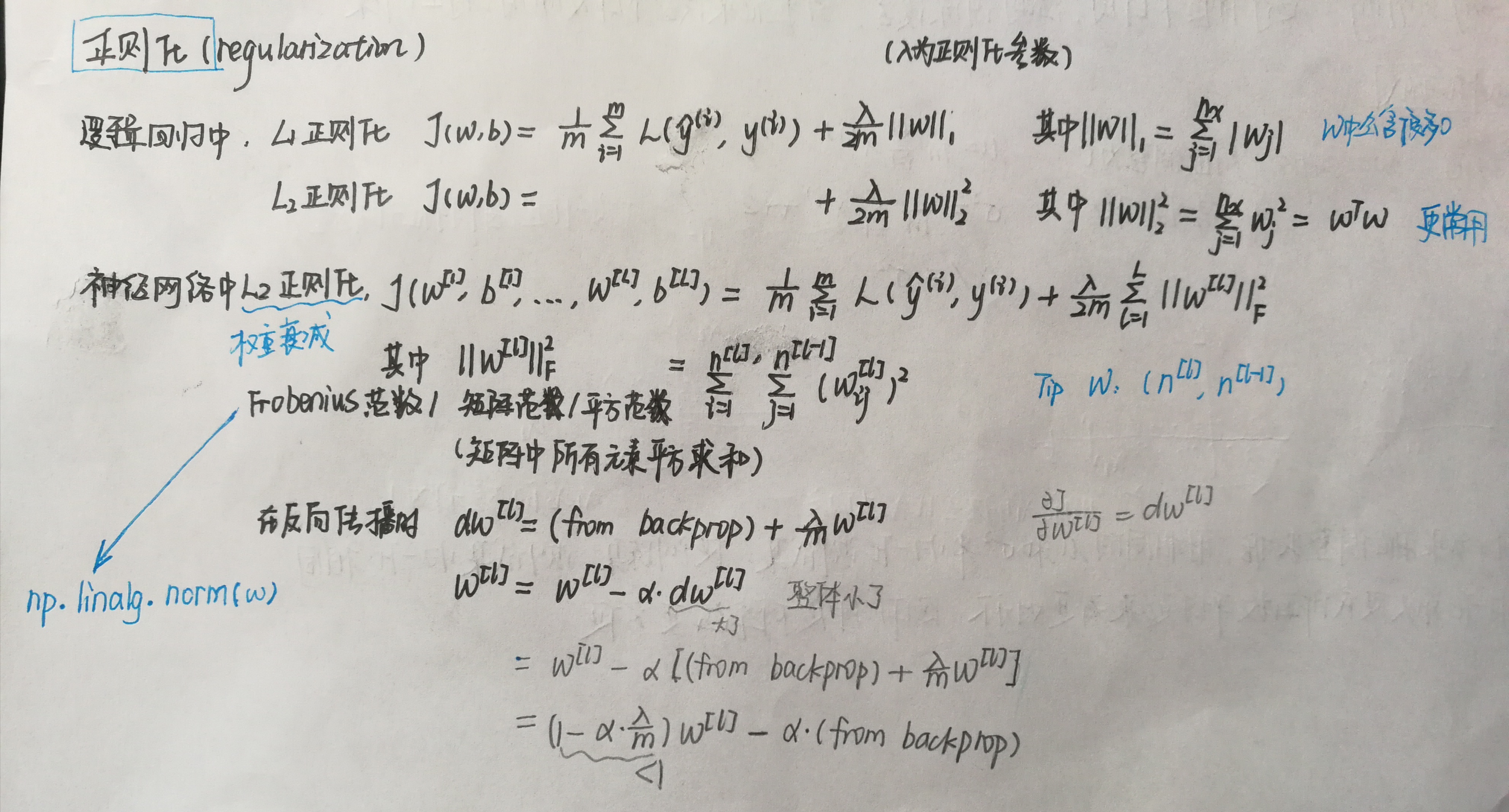
L2正则化
原始数据:
1 from reg_utils import sigmoid, relu, plot_decision_boundary, initialize_parameters, load_2D_dataset, predict_dec
2 from reg_utils import compute_cost, predict, forward_propagation, backward_propagation, update_parameters
3 import scipy.io
4 from testCases_v3 import *
5
6 train_X, train_Y, test_X, test_Y = load_2D_dataset()
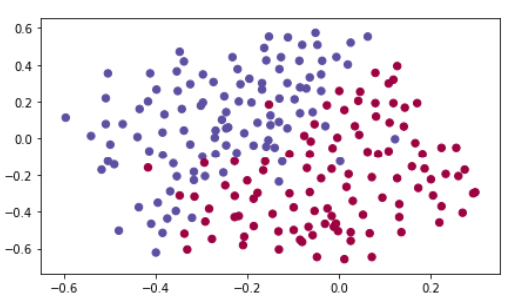
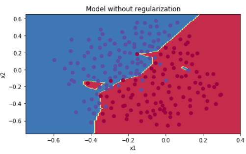
如果不使用正则化:
 1 def model(X, Y, learning_rate = 0.3, num_iterations = 30000, print_cost = True, lambd = 0, keep_prob = 1):
 2     """
 3     Implements a three-layer neural network: LINEAR->RELU->LINEAR->RELU->LINEAR->SIGMOID.
 4
 5     Arguments:
 6     X -- input data, of shape (input size, number of examples)
 7     Y -- true "label" vector (1 for blue dot / 0 for red dot), of shape (output size, number of examples)
 8     learning_rate -- learning rate of the optimization
 9     num_iterations -- number of iterations of the optimization loop
10     print_cost -- If True, print the cost every 10000 iterations
11     lambd -- regularization hyperparameter, scalar
12     keep_prob - probability of keeping a neuron active during drop-out, scalar.
13
14     Returns:
15     parameters -- parameters learned by the model. They can then be used to predict.
16     """
17
18     grads = {}
19     costs = []                            # to keep track of the cost
20     m = X.shape[1]                        # number of examples
21     layers_dims = [X.shape[0], 20, 3, 1]
22
23     # Initialize parameters dictionary.
24     parameters = initialize_parameters(layers_dims)
25
26     # Loop (gradient descent)
27     for i in range(0, num_iterations):
28
29         # Forward propagation: LINEAR -> RELU -> LINEAR -> RELU -> LINEAR -> SIGMOID.
30         if keep_prob == 1:
31             a3, cache = forward_propagation(X, parameters)
32         elif keep_prob < 1:
33             a3, cache = forward_propagation_with_dropout(X, parameters, keep_prob)
34
35         # Cost function
36         if lambd == 0:
37             cost = compute_cost(a3, Y)
38         else:
39             cost = compute_cost_with_regularization(a3, Y, parameters, lambd)
40
41         # Backward propagation.
42         assert(lambd == 0 or keep_prob == 1)    # it is possible to use both L2 regularization and dropout,
43                                             # but this assignment will only explore one at a time
44         if lambd == 0 and keep_prob == 1:
45             grads = backward_propagation(X, Y, cache)
46         elif lambd != 0:
47             grads = backward_propagation_with_regularization(X, Y, cache, lambd)
48         elif keep_prob < 1:
49             grads = backward_propagation_with_dropout(X, Y, cache, keep_prob)
50
51         # Update parameters.
52         parameters = update_parameters(parameters, grads, learning_rate)
53
54         # Print the loss every 10000 iterations
55         if print_cost and i % 10000 == 0:
56             print("Cost after iteration {}: {}".format(i, cost))
57         if print_cost and i % 1000 == 0:
58             costs.append(cost)
59
60     # plot the cost
61     plt.plot(costs)
62     plt.ylabel('cost')
63     plt.xlabel('iterations (x1,000)')
64     plt.title("Learning rate =" + str(learning_rate))
65     plt.show()
66
67     return parameters
68
69
70 parameters = model(train_X, train_Y)
71 print("On the training set:")
72 predictions_train = predict(train_X, train_Y, parameters)
73 print("On the test set:")
74 predictions_test = predict(test_X, test_Y, parameters)
75
76
77 plt.title("Model without regularization")
78 axes = plt.gca()
79 axes.set_xlim([-0.75, 0.40])
80 axes.set_ylim([-0.75, 0.65])
81 plot_decision_boundary(lambda x: predict_dec(parameters, x.T), train_X, train_Y)
预测准确度0.915
使用了L2正则化:
 1 # GRADED FUNCTION: compute_cost_with_regularization
 2 def compute_cost_with_regularization(A3, Y, parameters, lambd):
 3     """
 4     Implement the cost function with L2 regularization. See formula (2) above.
 5
 6     Arguments:
 7     A3 -- post-activation, output of forward propagation, of shape (output size, number of examples)
 8     Y -- "true" labels vector, of shape (output size, number of examples)
 9     parameters -- python dictionary containing parameters of the model
10
11     Returns:
12     cost - value of the regularized loss function (formula (2))
13     """
14     m = Y.shape[1]
15     W1 = parameters["W1"]
16     W2 = parameters["W2"]
17     W3 = parameters["W3"]
18
19     cross_entropy_cost = compute_cost(A3, Y) # This gives you the cross-entropy part of the cost
20
21     ### START CODE HERE ### (approx. 1 line)
22     L2_regularization_cost=lambd/(2*m)*(np.sum(np.square(W1)) + np.sum(np.square(W2))  + np.sum(np.square(W3)))
23     ### END CODER HERE ###
24
25     cost = cross_entropy_cost + L2_regularization_cost
26     return cost
27
28 A3, Y_assess, parameters = compute_cost_with_regularization_test_case()
29 print("cost = " + str(compute_cost_with_regularization(A3, Y_assess, parameters, lambd = 0.1)))
30
31
32 # GRADED FUNCTION: backward_propagation_with_regularization
33 def backward_propagation_with_regularization(X, Y, cache, lambd):
34     """
35     Implements the backward propagation of our baseline model to which we added an L2 regularization.
36
37     Arguments:
38     X -- input dataset, of shape (input size, number of examples)
39     Y -- "true" labels vector, of shape (output size, number of examples)
40     cache -- cache output from forward_propagation()
41     lambd -- regularization hyperparameter, scalar
42
43     Returns:
44     gradients -- A dictionary with the gradients with respect to each parameter, activation and pre-activation variables
45     """
46
47     m = X.shape[1]
48     (Z1, A1, W1, b1, Z2, A2, W2, b2, Z3, A3, W3, b3) = cache
49
50     dZ3 = A3 - Y
51
52     ### START CODE HERE ### (approx. 1 line)
53     dW3=np.dot(dZ3,A2.T)/m+lambd*W3/m
54     ### END CODE HERE ###
55     db3 = 1. / m * np.sum(dZ3, axis=1, keepdims=True)
56
57     dA2 = np.dot(W3.T, dZ3)
58     dZ2 = np.multiply(dA2, np.int64(A2 > 0))
59     ### START CODE HERE ### (approx. 1 line)
60     dW2=np.dot(dZ2,A1.T)/m+lambd*W2/m
61     ### END CODE HERE ###
62     db2 = 1. / m * np.sum(dZ2, axis=1, keepdims=True)
63
64     dA1 = np.dot(W2.T, dZ2)
65     dZ1 = np.multiply(dA1, np.int64(A1 > 0))
66     ### START CODE HERE ### (approx. 1 line)
67     dW1=np.dot(dZ1,X.T)/m+lambd*W1/m
68     ### END CODE HERE ###
69     db1 = 1. / m * np.sum(dZ1, axis=1, keepdims=True)
70
71     gradients = {"dZ3": dZ3, "dW3": dW3, "db3": db3, "dA2": dA2,
72                  "dZ2": dZ2, "dW2": dW2, "db2": db2, "dA1": dA1,
73                  "dZ1": dZ1, "dW1": dW1, "db1": db1}
74     return gradients
75
76
77 X_assess, Y_assess, cache = backward_propagation_with_regularization_test_case()
78 grads = backward_propagation_with_regularization(X_assess, Y_assess, cache, lambd=0.7)
79 print ("dW1 = " + str(grads["dW1"]))
80 print ("dW2 = " + str(grads["dW2"]))
81 print ("dW3 = " + str(grads["dW3"]))
82
83
84 parameters = model(train_X, train_Y, lambd=0.7)
85 print("On the train set:")
86 predictions_train = predict(train_X, train_Y, parameters)
87 print("On the test set:")
88 predictions_test = predict(test_X, test_Y, parameters)
89
90
91 plt.title("Model with L2-regularization")
92 axes = plt.gca()
93 axes.set_xlim([-0.75,0.40])
94 axes.set_ylim([-0.75,0.65])
95 plot_decision_boundary(lambda x: predict_dec(parameters, x.T), train_X, train_Y)
预测准确率0.93

Dropout正则化(随机失活)
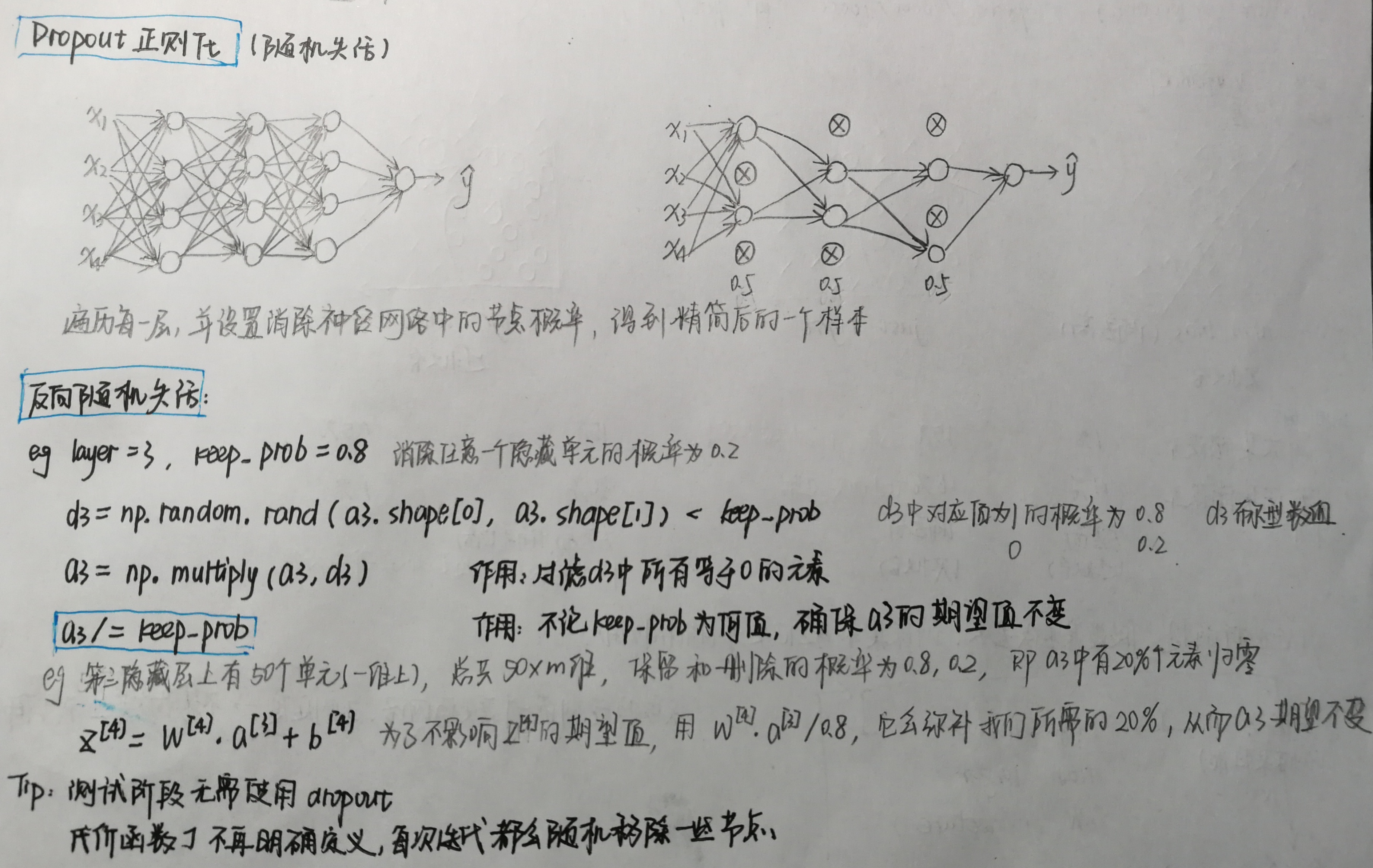
  1 # GRADED FUNCTION: forward_propagation_with_dropout
  2 def forward_propagation_with_dropout(X, parameters, keep_prob=0.5):
  3     """
  4     Implements the forward propagation: LINEAR -> RELU + DROPOUT -> LINEAR -> RELU + DROPOUT -> LINEAR -> SIGMOID.
  5
  6     Arguments:
  7     X -- input dataset, of shape (2, number of examples)
  8     parameters -- python dictionary containing your parameters "W1", "b1", "W2", "b2", "W3", "b3":
  9                     W1 -- weight matrix of shape (20, 2)
 10                     b1 -- bias vector of shape (20, 1)
 11                     W2 -- weight matrix of shape (3, 20)
 12                     b2 -- bias vector of shape (3, 1)
 13                     W3 -- weight matrix of shape (1, 3)
 14                     b3 -- bias vector of shape (1, 1)
 15     keep_prob - probability of keeping a neuron active during drop-out, scalar
 16
 17     Returns:
 18     A3 -- last activation value, output of the forward propagation, of shape (1,1)
 19     cache -- tuple, information stored for computing the backward propagation
 20     """
 21     np.random.seed(1)
 22
 23     # retrieve parameters
 24     W1 = parameters["W1"]
 25     b1 = parameters["b1"]
 26     W2 = parameters["W2"]
 27     b2 = parameters["b2"]
 28     W3 = parameters["W3"]
 29     b3 = parameters["b3"]
 30
 31     # LINEAR -> RELU -> LINEAR -> RELU -> LINEAR -> SIGMOID
 32     Z1 = np.dot(W1, X) + b1
 33     A1 = relu(Z1)
 34     ### START CODE HERE ### (approx. 4 lines)         # Steps 1-4 below correspond to the Steps 1-4 described above.
 35     D1=np.random.rand(A1.shape[0],A1.shape[1])        # Step 1: initialize matrix D1 = np.random.rand(..., ...)
 36     D1=D1<keep_prob                                   # Step 2: convert entries of D1 to 0 or 1 (using keep_prob as the threshold)
 37     A1=np.multiply(A1,D1)                             # Step 3: shut down some neurons of A1
 38     A1/=keep_prob                                     # Step 4: scale the value of neurons that haven't been shut down
 39     ### END CODE HERE ###
 40
 41     Z2 = np.dot(W2, A1) + b2
 42     A2 = relu(Z2)
 43     ### START CODE HERE ### (approx. 4 lines)
 44     D2=np.random.rand(A2.shape[0], A2.shape[1])      # Step 1: initialize matrix D2 = np.random.rand(..., ...)
 45     D2=D2<keep_prob                                  # Step 2: convert entries of D2 to 0 or 1 (using keep_prob as the threshold)
 46     A2=np.multiply(A2,D2)                            # Step 3: shut down some neurons of A2
 47     A2/=keep_prob                                    # Step 4: scale the value of neurons that haven't been shut down
 48     ### END CODE HERE ###
 49
 50     Z3 = np.dot(W3, A2) + b3
 51     A3 = sigmoid(Z3)
 52
 53     cache = (Z1, D1, A1, W1, b1, Z2, D2, A2, W2, b2, Z3, A3, W3, b3)
 54     return A3, cache
 55
 56 X_assess, parameters = forward_propagation_with_dropout_test_case()
 57 A3, cache = forward_propagation_with_dropout(X_assess, parameters, keep_prob=0.7)
 58 print ("A3 = " + str(A3))
 59
 60
 61 # GRADED FUNCTION: backward_propagation_with_dropout
 62 def backward_propagation_with_dropout(X, Y, cache, keep_prob):
 63     """
 64     Implements the backward propagation of our baseline model to which we added dropout.
 65
 66     Arguments:
 67     X -- input dataset, of shape (2, number of examples)
 68     Y -- "true" labels vector, of shape (output size, number of examples)
 69     cache -- cache output from forward_propagation_with_dropout()
 70     keep_prob - probability of keeping a neuron active during drop-out, scalar
 71
 72     Returns:
 73     gradients -- A dictionary with the gradients with respect to each parameter, activation and pre-activation variables
 74     """
 75
 76     m = X.shape[1]
 77     (Z1, D1, A1, W1, b1, Z2, D2, A2, W2, b2, Z3, A3, W3, b3) = cache
 78
 79     dZ3 = A3 - Y
 80     dW3 = 1. / m * np.dot(dZ3, A2.T)
 81     db3 = 1. / m * np.sum(dZ3, axis=1, keepdims=True)
 82
 83     dA2 = np.dot(W3.T, dZ3)
 84     ### START CODE HERE ### (≈ 2 lines of code)
 85     dA2 = dA2*D2               # Step 1: Apply mask D2 to shut down the same neurons as during the forward propagation
 86     dA2 = dA2/keep_prob        # Step 2: Scale the value of neurons that haven't been shut down
 87     ### END CODE HERE ###
 88
 89     dZ2 = np.multiply(dA2, np.int64(A2 > 0))
 90     dW2 = 1. / m * np.dot(dZ2, A1.T)
 91     db2 = 1. / m * np.sum(dZ2, axis=1, keepdims=True)
 92
 93     dA1 = np.dot(W2.T, dZ2)
 94     ### START CODE HERE ### (≈ 2 lines of code)
 95     dA1=dA1*D1                   # Step 1: Apply mask D1 to shut down the same neurons as during the forward propagation
 96     dA1=dA1/keep_prob            # Step 2: Scale the value of neurons that haven't been shut down
 97     ### END CODE HERE ###
 98
 99     dZ1 = np.multiply(dA1, np.int64(A1 > 0))
100     dW1 = 1. / m * np.dot(dZ1, X.T)
101     db1 = 1. / m * np.sum(dZ1, axis=1, keepdims=True)
102
103     gradients = {"dZ3": dZ3, "dW3": dW3, "db3": db3,"dA2": dA2,
104                  "dZ2": dZ2, "dW2": dW2, "db2": db2, "dA1": dA1,
105                  "dZ1": dZ1, "dW1": dW1, "db1": db1}
106
107     return gradients
108
109
110 X_assess, Y_assess, cache = backward_propagation_with_dropout_test_case()
111 gradients = backward_propagation_with_dropout(X_assess, Y_assess, cache, keep_prob=0.8)
112 print ("dA1 = " + str(gradients["dA1"]))
113 print ("dA2 = " + str(gradients["dA2"]))
114
115
116 parameters = model(train_X, train_Y, keep_prob=0.86, learning_rate=0.3)
117 print("On the train set:")
118 predictions_train = predict(train_X, train_Y, parameters)
119 print("On the test set:")
120 predictions_test = predict(test_X, test_Y, parameters)
121
122
123 plt.title("Model with dropout")
124 axes = plt.gca()
125 axes.set_xlim([-0.75, 0.40])
126 axes.set_ylim([-0.75, 0.65])
127 plot_decision_boundary(lambda x: predict_dec(parameters, x.T), train_X, train_Y)
预测准确度0.95

梯度校验

一维梯度校验:
 1 from testCases_v3 import gradient_check_n_test_case
 2 from gc_utils import sigmoid, relu, dictionary_to_vector, vector_to_dictionary, gradients_to_vector
 3
 4 #一维梯度校验
 5 # GRADED FUNCTION: forward_propagation
 6 def forward_propagation(x, theta):
 7     """
 8     Implement the linear forward propagation (compute J) presented in Figure 1 (J(theta) = theta * x)
 9
10     Arguments:
11     x -- a real-valued input
12     theta -- our parameter, a real number as well
13
14     Returns:
15     J -- the value of function J, computed using the formula J(theta) = theta * x
16     """
17
18     ### START CODE HERE ### (approx. 1 line)
19     J = np.dot(theta, x)
20     ### END CODE HERE ###
21     return J
22
23 x, theta = 2, 4
24 J = forward_propagation(x, theta)
25 print ("J = " + str(J))
26
27
28 # GRADED FUNCTION: backward_propagation
29 def backward_propagation(x, theta):
30     """
31     Computes the derivative of J with respect to theta (see Figure 1).
32
33     Arguments:
34     x -- a real-valued input
35     theta -- our parameter, a real number as well
36
37     Returns:
38     dtheta -- the gradient of the cost with respect to theta
39     """
40     ### START CODE HERE ### (approx. 1 line)
41     dtheta=x
42     ### END CODE HERE ###
43     return dtheta
44
45 x, theta = 2, 4
46 dtheta = backward_propagation(x, theta)
47 print ("dtheta = " + str(dtheta))
48
49
50 # GRADED FUNCTION: gradient_check
51 def gradient_check(x, theta, epsilon=1e-7):
52     """
53     Implement the backward propagation presented in Figure 1.
54
55     Arguments:
56     x -- a real-valued input
57     theta -- our parameter, a real number as well
58     epsilon -- tiny shift to the input to compute approximated gradient with formula(1)
59
60     Returns:
61     difference -- difference (2) between the approximated gradient and the backward propagation gradient
62     """
63
64     # Compute gradapprox using left side of formula (1). epsilon is small enough, you don't need to worry about the limit.
65     ### START CODE HERE ### (approx. 5 lines)
66     theta1=theta+epsilon                              # Step 1
67     theta2=theta-epsilon                              # Step 2
68     J1=forward_propagation(x, theta1)                 # Step 3
69     J2=forward_propagation(x, theta2)                 # Step 4
70     gradapprox=(J1-J2)/(2*epsilon)                    # Step 5
71     ### END CODE HERE ###
72
73     # Check if gradapprox is close enough to the output of backward_propagation()
74     ### START CODE HERE ### (approx. 1 line)
75     grad = backward_propagation(x, theta)
76     ### END CODE HERE ###
77
78     ### START CODE HERE ### (approx. 1 line)
79     numerator = np.linalg.norm(grad - gradapprox)                      # Step 1'
80     denominator = np.linalg.norm(grad) + np.linalg.norm(gradapprox)    # Step 2'
81     difference = numerator / denominator                               # Step 3'
82     ### END CODE HERE ###
83
84     if difference < 1e-7:
85         print("The gradient is correct!")
86     else:
87         print("The gradient is wrong!")
88
89     return difference
90
91 x, theta = 2, 4
92 difference = gradient_check(x, theta)
93 print("difference = " + str(difference))
输出:
The gradient is correct!
difference = 2.919335883291695e-10
N维梯度校验:
1 #N维梯度校验 2 def forward_propagation_n(X, Y, parameters): 3 """ 4 Implements the forward propagation (and computes the cost) presented in Figure 3. 5 6 Arguments: 7 X -- training set for m examples 8 Y -- labels for m examples 9 parameters -- python dictionary containing your parameters "W1", "b1", "W2", "b2", "W3", "b3": 10 W1 -- weight matrix of shape (5, 4) 11 b1 -- bias vector of shape (5, 1) 12 W2 -- weight matrix of shape (3, 5) 13 b2 -- bias vector of shape (3, 1) 14 W3 -- weight matrix of shape (1, 3) 15 b3 -- bias vector of shape (1, 1) 16 17 Returns: 18 cost -- the cost function (logistic cost for one example) 19 """ 20 21 # retrieve parameters 22 m = X.shape[1] 23 W1 = parameters["W1"] 24 b1 = parameters["b1"] 25 W2 = parameters["W2"] 26 b2 = parameters["b2"] 27 W3 = parameters["W3"] 28 b3 = parameters["b3"] 29 30 # LINEAR -> RELU -> LINEAR -> RELU -> LINEAR -> SIGMOID 31 Z1 = np.dot(W1, X) + b1 32 A1 = relu(Z1) 33 Z2 = np.dot(W2, A1) + b2 34 A2 = relu(Z2) 35 Z3 = np.dot(W3, A2) + b3 36 A3 = sigmoid(Z3) 37 38 # Cost 39 logprobs = np.multiply(-np.log(A3), Y) + np.multiply(-np.log(1 - A3), 1 - Y) 40 cost = 1. / m * np.sum(logprobs) 41 42 cache = (Z1, A1, W1, b1, Z2, A2, W2, b2, Z3, A3, W3, b3) 43 44 return cost, cache 45 46 47 def backward_propagation_n(X, Y, cache): 48 """ 49 Implement the backward propagation presented in figure 2. 50 51 Arguments: 52 X -- input datapoint, of shape (input size, 1) 53 Y -- true "label" 54 cache -- cache output from forward_propagation_n() 55 56 Returns: 57 gradients -- A dictionary with the gradients of the cost with respect to each parameter, activation and pre-activation variables. 58 """ 59 60 m = X.shape[1] 61 (Z1, A1, W1, b1, Z2, A2, W2, b2, Z3, A3, W3, b3) = cache 62 63 dZ3 = A3 - Y 64 dW3 = 1. / m * np.dot(dZ3, A2.T) 65 db3 = 1. / m * np.sum(dZ3, axis=1, keepdims=True) 66 67 dA2 = np.dot(W3.T, dZ3) 68 dZ2 = np.multiply(dA2, np.int64(A2 > 0)) 69 dW2 = 1. / m * np.dot(dZ2, A1.T) * 2 # Should not multiply by 2 70 db2 = 1. / m * np.sum(dZ2, axis=1, keepdims=True) 71 72 dA1 = np.dot(W2.T, dZ2) 73 dZ1 = np.multiply(dA1, np.int64(A1 > 0)) 74 dW1 = 1. / m * np.dot(dZ1, X.T) 75 db1 = 4. / m * np.sum(dZ1, axis=1, keepdims=True) # Should not multiply by 4 76 77 gradients = {"dZ3": dZ3, "dW3": dW3, "db3": db3, 78 "dA2": dA2, "dZ2": dZ2, "dW2": dW2, "db2": db2, 79 "dA1": dA1, "dZ1": dZ1, "dW1": dW1, "db1": db1} 80 81 return gradients 82 83 84 # GRADED FUNCTION: gradient_check_n 85 def gradient_check_n(parameters, gradients, X, Y, epsilon=1e-7): 86 """ 87 Checks if backward_propagation_n computes correctly the gradient of the cost output by forward_propagation_n 88 89 Arguments: 90 parameters -- python dictionary containing your parameters "W1", "b1", "W2", "b2", "W3", "b3": 91 grad -- output of backward_propagation_n, contains gradients of the cost with respect to the parameters. 92 x -- input datapoint, of shape (input size, 1) 93 y -- true "label" 94 epsilon -- tiny shift to the input to compute approximated gradient with formula(1) 95 96 Returns: 97 difference -- difference (2) between the approximated gradient and the backward propagation gradient 98 """ 99 100 # Set-up variables 101 parameters_values, _ = dictionary_to_vector(parameters) 102 grad = gradients_to_vector(gradients) 103 num_parameters = parameters_values.shape[0] 104 J_plus = np.zeros((num_parameters, 1)) 105 J_minus = np.zeros((num_parameters, 1)) 106 gradapprox = np.zeros((num_parameters, 1)) 107 108 # Compute gradapprox 109 for i in range(num_parameters): 110 111 # Compute J_plus[i]. Inputs: "parameters_values, epsilon". Output = "J_plus[i]". 112 # "_" is used because the function you have to outputs two parameters but we only care about the first one 113 ### START CODE HERE ### (approx. 3 lines) 114 theta1=np.copy(parameters_values) # Step 1 115 theta1[i][0]+=epsilon # Step 2 116 J_plus[i],_=forward_propagation_n(X, Y, vector_to_dictionary(theta1)) # Step 3 117 ### END CODE HERE ### 118 119 120 # Compute J_minus[i]. Inputs: "parameters_values, epsilon". Output = "J_minus[i]". 121 ### START CODE HERE ### (approx. 3 lines) 122 theta2=np.copy(parameters_values) # Step 1 123 theta2[i][0]-=epsilon # Step 2 124 J_minus[i],_=forward_propagation_n(X, Y, vector_to_dictionary(theta2)) # Step 3 125 ### END CODE HERE ### 126 127 # Compute gradapprox[i] 128 ### START CODE HERE ### (approx. 1 line) 129 gradapprox[i]=(J_plus[i]-J_minus[i])/(2*epsilon) 130 ### END CODE HERE ### 131 132 # Compare gradapprox to backward propagation gradients by computing difference. 133 ### START CODE HERE ### (approx. 1 line) 134 numerator = np.linalg.norm(grad - gradapprox) # Step 1' 135 denominator = np.linalg.norm(grad) + np.linalg.norm(gradapprox) # Step 2' 136 difference = numerator / denominator # Step 3' 137 ### END CODE HERE ### 138 139 if difference > 1e-7: 140 print("�33[93m" + "There is a mistake in the backward propagation! difference = " + str(difference) + "�33[0m") 141 else: 142 print("�33[92m" + "Your backward propagation works perfectly fine! difference = " + str(difference) + "�33[0m") 143 144 return difference 145 146 147 X, Y, parameters = gradient_check_n_test_case() 148 149 cost, cache = forward_propagation_n(X, Y, parameters) 150 gradients = backward_propagation_n(X, Y, cache) 151 difference = gradient_check_n(parameters, gradients, X, Y)
输出:
There is a mistake in the backward propagation! difference = 0.2850931566540251