理论知识:Optimization: Stochastic Gradient Descent和Convolutional Neural Network
CNN卷积神经网络推导和实现、Deep learning:五十一(CNN的反向求导及练习)
Deep Learning 学习随记(八)CNN(Convolutional neural network)理解
ufldl学习笔记与编程作业:Convolutional Neural Network(卷积神经网络)
【UFLDL】Exercise: Convolutional Neural Network
基础知识
下面是Convolutional Neural Network的翻译
概述
CNN是由一个或多个卷积层(其后常跟一个下采样层)和一个或多个全连接层组成的多层神经网络。CNN的输入是2维图像(或者其他2维输入,如语音信号)。它通过局部连接和权值共享,再通过池化可得到平移不变特征。CNN的另一个优点就是易于训练,相比同样隐含层单元的全连接网络,它需要训练的参数个数要少得多。本文将介绍CNN的结构和后向传播算法,该算法用于计算对模型参数的梯度。卷积和池化可看前面相应的教程。
结构
CNN由一些卷积层和下采样层交替组成,也可视需要在最后加全连接层。一个卷积层的输入是m*m*r的图像,其中m是图像的高度和宽度,r是通道数,如RGB图像的r=3。卷积层有k个滤波器(或核函数),大小为n*n*q,其中n小于图像的维数,q小于等于r且每个滤波器的q可能不一样。滤波器的大小产生局部连接结构,该结构是由每个滤波器与输入图像卷积得到k个特征图,每个特征图大小为m-n+1。然后,每个特征图通过p*p连续区域的平均或最大池化的方式来子采样,其中p一般取2(当输入为小图像时,如MNIST)和5(当输入是大图像时)之间。在子采样层的前后均需对每个特征图加一个附加偏置项和sigmoid非线性变化。下图显示了一个由卷积层和子采样层组成的CNN。其中,相同颜色的单元共享权值。
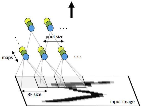
图1.卷积神经网络的带池化的第一层。相同颜色的神经元共享权值,不同颜色神经元表示不同的特征图。
在卷积层的最后可能会有一些全连接层。该层是与一个标准多层神经网络中的层是一样的。
后向传播
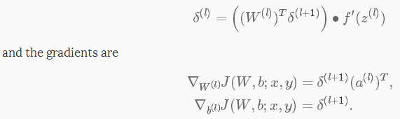
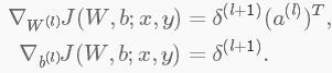
δ(l+1)中是l+1层的残差,代价函数为J(W,b;x,y),其中(W,b)是参数,(x,y)分别是训练数据和标签。则l层的残差和梯度分别为:
如果l层是一个卷积层和子采样层,则其残差为:

其中,k是滤波器个数, 是激活函数的偏层数。通过计算传入池化层每个神经元的残差,子采样必须通过池化层传播残差。
最后,为了计算特征图的梯度,利用边缘处理卷积运算得到残差矩阵,再翻转残差矩阵。在卷积层翻转滤波器和最后翻转残差矩阵效果是一样的。
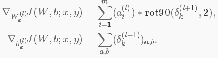
其中,
a(L)是L层的输入,a(1)是输入图像。 是一个合理的卷积运算,该卷积是第l层的第i个输入与对第k个滤波器的残差相卷。
练习
练习内容:UFLDL:Exercise: Convolutional Neural Network。利用卷积神经网络实现数字分类。该神经网络有2层,第一层是卷积和子采样层,第二层是全连接层。即:本节的网络结构为:一个卷积层+一个pooling层+一个softmax层。本节练习中,输入图像为28*28,卷积核大小为9*9,卷积层特征个数(即:卷积核个数)为20个,池化连续区域为2*2,输出为类别为10类。
参考:【UFLDL】Exercise: Convolutional Neural Network讲解非常详细
注意:本练习中的卷积核,并不是由自编码器学习的特征,而是随机随机始化所得
一些matlab函数
1.addpath
语法:
添加路径:addpath('当前路径中的文件夹名1','当前路径下的文件夹名2','当前路径中的文件夹名n');【即可一次性添加多个路径】
addpath('./上级目录中的文件夹1','./上级目录中的文件夹2','./上级目录中的文件夹n');
addpath('../更上一级目录中的文件夹1','../更上一级目录中的文件夹2','../更上一级目录中的文件夹n');
3.sub2ind函数
ind2sub函数可以用来把矩阵元素的index转换成对应的下标(determines the equivalent subscript values corresponding to a single index into an array)
例如: 一个4*5的矩阵A,第2行第2个元素的index的6(matlab中matrix是按列顺序排列),可以用ind2sub函数来计算这个元素的下标 [I,J] = ind2sub(size(A),6)
4.sparse和full函数
见Deep Learning 6_深度学习UFLDL教程:Softmax Regression_Exercise(斯坦福大学深度学习教程)
下面这句话经常可见:
groundTruth = full(sparse(labels, 1:numImages, 1));
它得到的结果是这样一个矩阵:在第i行第j列元素值为1,其他元素为0,其中,i是向量labels内的第k个元素值,j是向量1:numImages内的第k个元素值。
故,在cnnCost.m中计算cost的代码为:
logProbs = log(probs);
labelIndex=sub2ind(size(logProbs), labels', 1:size(logProbs,2));
%找出矩阵logProbs的线性索引,行由labels指定,列由1:size(logProbs,2)指定,生成线性索引返回给labelIndex
values = logProbs(labelIndex);
cost = -sum(values);
weightDecayCost = (weightDecay/2) * (sum(Wd(:) .^ 2) + sum(Wc(:) .^ 2));
cost = cost / numImages+weightDecayCost;
可把它替换为:
groundTruth = full(sparse(labels, 1:numImages, 1));
cost = -1./numImages*groundTruth(:)'*log(probs(:))+(weightDecay/2.)*(sum(Wd(:).^2)+sum(Wc(:).^2)); %加入一个惩罚项
变得效率更快,代码更简洁。
练习步骤
STEP 1:实现CNN代价函数和梯度计算
STEP 1a: Forward Propagation
STEP 1b: Calculate Cost
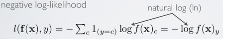
代价函数:

其中,J(W,b)为:
STEP 1c: Backpropagation
softmax 层误差:softmaxError,见Deep learning:五十一(CNN的反向求导及练习)
pool 层误差:poolError,这一层首先根据公式δl = Wδl+1 * f'(zl)(pool层没有f'(zl)这一项)计算该层的error。即poolError为:δl = Wδl+1
展开poolError为unpoolError,
convolution层误差:convError,还是根据公式δl = Wδl+1 * f'(zl)来计算
STEP 1d: Gradient Calculation
Wd和bd的梯度计算公式:
Step 2: Gradient Check
非常重要的一步
Step 3: Learn Parameters
在minFuncSGD中加上冲量的影响即可。
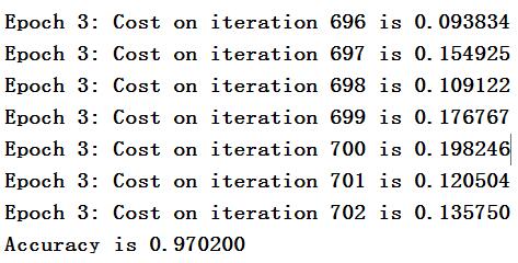
Step 4: Test
结果为:
代码
cnnTrain.m
%% Convolution Neural Network Exercise

%  Instructions
%  ------------
%
%  This file contains code that helps you get started in building a single.
%  layer convolutional nerual network. In this exercise, you will only
%  need to modify cnnCost.m and cnnminFuncSGD.m. You will not need to
%  modify this file.

%%======================================================================
%% STEP 0: Initialize Parameters and Load Data
%  Here we initialize some parameters used for the exercise.

% Configuration
imageDim = 28;
numClasses = 10;  % Number of classes (MNIST images fall into 10 classes)
filterDim = 9;    % Filter size for conv layer,9*9
numFilters = 20;   % Number of filters for conv layer
poolDim = 2;      % Pooling dimension, (should divide imageDim-filterDim+1)

% Load MNIST Train
addpath ../common/;
images = loadMNISTImages('../common/train-images-idx3-ubyte');
images = reshape(images,imageDim,imageDim,[]);
labels = loadMNISTLabels('../common/train-labels-idx1-ubyte');
labels(labels==0) = 10; % Remap 0 to 10

% Initialize Parameters,theta=(2165,1),2165=9*9*20+20+100*20*10+10
theta = cnnInitParams(imageDim,filterDim,numFilters,poolDim,numClasses);

%%======================================================================
%% STEP 1: Implement convNet Objective
%  Implement the function cnnCost.m.

%%======================================================================
%% STEP 2: Gradient Check
%  Use the file computeNumericalGradient.m to check the gradient
%  calculation for your cnnCost.m function.  You may need to add the
%  appropriate path or copy the file to this directory.

% DEBUG=false;  % set this to true to check gradient
DEBUG = true;
if DEBUG
    % To speed up gradient checking, we will use a reduced network and
    % a debugging data set
    db_numFilters = 2;
    db_filterDim = 9;
    db_poolDim = 5;
    db_images = images(:,:,1:10);
    db_labels = labels(1:10);
    db_theta = cnnInitParams(imageDim,db_filterDim,db_numFilters,...
                db_poolDim,numClasses);

    [cost grad] = cnnCost(db_theta,db_images,db_labels,numClasses,...
                                db_filterDim,db_numFilters,db_poolDim);


    % Check gradients
    numGrad = computeNumericalGradient( @(x) cnnCost(x,db_images,...
                                db_labels,numClasses,db_filterDim,...
                                db_numFilters,db_poolDim), db_theta);

    % Use this to visually compare the gradients side by side
    disp([numGrad grad]);

    diff = norm(numGrad-grad)/norm(numGrad+grad);
    % Should be small. In our implementation, these values are usually
    % less than 1e-9.
    disp(diff);

    assert(diff < 1e-9,...
        'Difference too large. Check your gradient computation again');

end;

%%======================================================================
%% STEP 3: Learn Parameters
%  Implement minFuncSGD.m, then train the model.

% 因为是采用的mini-batch梯度下降法,所以总共对样本的循环次数次数比标准梯度下降法要少
% 很多,因为每次循环中权值已经迭代多次了
options.epochs = 3;
options.minibatch = 256;
options.alpha = 1e-1;
options.momentum = .95;

opttheta = minFuncSGD(@(x,y,z) cnnCost(x,y,z,numClasses,filterDim,...
                      numFilters,poolDim),theta,images,labels,options);
save('theta.mat','opttheta');

%%======================================================================
%% STEP 4: Test
%  Test the performance of the trained model using the MNIST test set. Your
%  accuracy should be above 97% after 3 epochs of training

testImages = loadMNISTImages('../common/t10k-images-idx3-ubyte');
testImages = reshape(testImages,imageDim,imageDim,[]);
testLabels = loadMNISTLabels('../common/t10k-labels-idx1-ubyte');
testLabels(testLabels==0) = 10; % Remap 0 to 10

[~,cost,preds]=cnnCost(opttheta,testImages,testLabels,numClasses,...
                filterDim,numFilters,poolDim,true);

acc = sum(preds==testLabels)/length(preds);

% Accuracy should be around 97.4% after 3 epochs
fprintf('Accuracy is %f
',acc);
cnnCost.m
function [cost, grad, preds] = cnnCost(theta,images,labels,numClasses,...
                filterDim,numFilters,poolDim,pred)
% Calcualte cost and gradient for a single layer convolutional
% neural network followed by a softmax layer with cross entropy
% objective.
%
% Parameters:
%  theta      -  unrolled parameter vector
%  images     -  stores images in imageDim x imageDim x numImges
%                array
%  numClasses -  number of classes to predict
%  filterDim  -  dimension of convolutional filter
%  numFilters -  number of convolutional filters
%  poolDim    -  dimension of pooling area
%  pred       -  boolean only forward propagate and return
%                predictions
%
%
% Returns:
%  cost       -  cross entropy cost
%  grad       -  gradient with respect to theta (if pred==False)
%  preds      -  list of predictions for each example (if pred==True)


if ~exist('pred','var')
  pred = false;
end;

weightDecay = 0.0001;

imageDim = size(images,1); % height/width of image
numImages = size(images,3); % number of images

%% Reshape parameters and setup gradient matrices

% Wc is filterDim x filterDim x numFilters parameter matrix %convolution参数
% bc is the corresponding bias

% Wd is numClasses x hiddenSize parameter matrix where hiddenSize
% is the number of output units from the convolutional layer %这个convolutional layer应该是包含了卷积层和pool层
% bd is corresponding bias
[Wc, Wd, bc, bd] = cnnParamsToStack(theta,imageDim,filterDim,numFilters,...
            poolDim,numClasses);

% Same sizes as Wc,Wd,bc,bd. Used to hold gradient w.r.t above params.
Wc_grad = zeros(size(Wc));
Wd_grad = zeros(size(Wd));
bc_grad = zeros(size(bc));
bd_grad = zeros(size(bd));

%%======================================================================
%% STEP 1a: Forward Propagation
%  In this step you will forward propagate the input through the
%  convolutional and subsampling (mean pooling) layers.  You will then use
%  the responses from the convolution and pooling layer as the input to a
%  standard softmax layer.

%% Convolutional Layer
%  For each image and each filter, convolve the image with the filter, add
%  the bias and apply the sigmoid nonlinearity.  Then subsample the
%  convolved activations with mean pooling.  Store the results of the
%  convolution in activations and the results of the pooling in
%  activationsPooled.  You will need to save the convolved activations for
%  backpropagation.
convDim = imageDim-filterDim+1; % dimension of convolved output
outputDim = (convDim)/poolDim; % dimension of subsampled output

% convDim x convDim x numFilters x numImages tensor for storing activations
activations = zeros(convDim,convDim,numFilters,numImages);

% outputDim x outputDim x numFilters x numImages tensor for storing
% subsampled activations
activationsPooled = zeros(outputDim,outputDim,numFilters,numImages);

%%% YOUR CODE HERE %%%   %调用之前写的两个函数
activations = cnnConvolve(filterDim, numFilters, images, Wc, bc);
activationsPooled = cnnPool(poolDim, activations);


% Reshape activations into 2-d matrix, hiddenSize x numImages,
% for Softmax layer
activationsPooled = reshape(activationsPooled,[],numImages);%就变成了传统的softmax模式

%% Softmax Layer
%  Forward propagate the pooled activations calculated above into a
%  standard softmax layer. For your convenience we have reshaped
%  activationPooled into a hiddenSize x numImages matrix.  Store the
%  results in probs.

% numClasses x numImages for storing probability that each image belongs to
% each class.
probs = zeros(numClasses,numImages);

%%% YOUR CODE HERE %%%
z = Wd*activationsPooled;
z = bsxfun(@plus,z,bd);
%z = Wd * activationsPooled+repmat(bd,[1,numImages]);
z = bsxfun(@minus,z,max(z,[],1));%减去最大值,减少一个维度,防止溢出
z = exp(z);
probs = bsxfun(@rdivide,z,sum(z,1));
preds = probs;
%%======================================================================
%% STEP 1b: Calculate Cost
%  In this step you will use the labels given as input and the probs
%  calculate above to evaluate the cross entropy objective.  Store your
%  results in cost.

cost = 0; % save objective into cost

%%% YOUR CODE HERE %%%
logProbs = log(probs);
labelIndex=sub2ind(size(logProbs), labels', 1:size(logProbs,2));
%找出矩阵logProbs的线性索引,行由labels指定,列由1:size(logProbs,2)指定,生成线性索引返回给labelIndex
values = logProbs(labelIndex);
cost = -sum(values);
weightDecayCost = (weightDecay/2) * (sum(Wd(:) .^ 2) + sum(Wc(:) .^ 2));
cost = cost / numImages+weightDecayCost;
%Make sure to scale your gradients by the inverse size of the training set
%if you included this scale in the cost calculation otherwise your code will not pass the numerical gradient check.


% Makes predictions given probs and returns without backproagating errors.
if pred
  [~,preds] = max(probs,[],1);
  preds = preds';
  grad = 0;
  return;
end;


%%======================================================================
%% STEP 1c: Backpropagation
%  Backpropagate errors through the softmax and convolutional/subsampling
%  layers.  Store the errors for the next step to calculate the gradient.
%  Backpropagating the error w.r.t the softmax layer is as usual.  To
%  backpropagate through the pooling layer, you will need to upsample the
%  error with respect to the pooling layer for each filter and each image.
%  Use the kron function and a matrix of ones to do this upsampling
%  quickly.

%%% YOUR CODE HERE %%%
%softmax残差
targetMatrix = zeros(size(probs));
targetMatrix(labelIndex) = 1;
softmaxError = probs-targetMatrix;

%pool层残差
poolError = Wd'*softmaxError;
poolError = reshape(poolError, outputDim, outputDim, numFilters, numImages);

unpoolError = zeros(convDim, convDim, numFilters, numImages);
unpoolingFilter = ones(poolDim);
poolArea = poolDim*poolDim;
%展开poolError为unpoolError
for imageNum = 1:numImages
  for filterNum = 1:numFilters
    e = poolError(:, :, filterNum, imageNum);
    unpoolError(:, :, filterNum, imageNum) = kron(e, unpoolingFilter)./poolArea;
  end
end

convError = unpoolError .* activations .* (1 - activations);


%%======================================================================
%% STEP 1d: Gradient Calculation
%  After backpropagating the errors above, we can use them to calculate the
%  gradient with respect to all the parameters.  The gradient w.r.t the
%  softmax layer is calculated as usual.  To calculate the gradient w.r.t.
%  a filter in the convolutional layer, convolve the backpropagated error
%  for that filter with each image and aggregate over images.

%%% YOUR CODE HERE %%%
%softmax梯度
Wd_grad = (1/numImages).*softmaxError * activationsPooled'+weightDecay * Wd; % l+1层残差 * l层激活值
bd_grad = (1/numImages).*sum(softmaxError, 2);

% Gradient of the convolutional layer
bc_grad = zeros(size(bc));
Wc_grad = zeros(size(Wc));

%计算bc_grad
for filterNum = 1 : numFilters
  e = convError(:, :, filterNum, :);
  bc_grad(filterNum) = (1/numImages).*sum(e(:));
end

%翻转convError
for filterNum = 1 : numFilters
  for imageNum = 1 : numImages
    e = convError(:, :, filterNum, imageNum);
    convError(:, :, filterNum, imageNum) = rot90(e, 2);
  end
end

for filterNum = 1 : numFilters
  Wc_gradFilter = zeros(size(Wc_grad, 1), size(Wc_grad, 2));
  for imageNum = 1 : numImages
    Wc_gradFilter = Wc_gradFilter + conv2(images(:, :, imageNum), convError(:, :, filterNum, imageNum), 'valid');
  end
  Wc_grad(:, :, filterNum) = (1/numImages).*Wc_gradFilter;
end
Wc_grad = Wc_grad + weightDecay * Wc;

%% Unroll gradient into grad vector for minFunc
grad = [Wc_grad(:) ; Wd_grad(:) ; bc_grad(:) ; bd_grad(:)];

end
cnnConvolve.m
function convolvedFeatures = cnnConvolve(filterDim, numFilters, images, W, b)
%cnnConvolve Returns the convolution of the features given by W and b with
%the given images
%
% Parameters:
%  filterDim - filter (feature) dimension
%  numFilters - number of feature maps
%  images - large images to convolve with, matrix in the form
%           images(r, c, image number)
%  W, b - W, b for features from the sparse autoencoder
%         W is of shape (filterDim,filterDim,numFilters)
%         b is of shape (numFilters,1)
%
% Returns:
%  convolvedFeatures - matrix of convolved features in the form
%                      convolvedFeatures(imageRow, imageCol, featureNum, imageNum)

numImages = size(images, 3);
imageDim = size(images, 1);
convDim = imageDim - filterDim + 1;

convolvedFeatures = zeros(convDim, convDim, numFilters, numImages);

% Instructions:
%   Convolve every filter with every image here to produce the
%   (imageDim - filterDim + 1) x (imageDim - filterDim + 1) x numFeatures x numImages
%   matrix convolvedFeatures, such that
%   convolvedFeatures(imageRow, imageCol, featureNum, imageNum) is the
%   value of the convolved featureNum feature for the imageNum image over
%   the region (imageRow, imageCol) to (imageRow + filterDim - 1, imageCol + filterDim - 1)
%
% Expected running times:
%   Convolving with 100 images should take less than 30 seconds
%   Convolving with 5000 images should take around 2 minutes
%   (So to save time when testing, you should convolve with less images, as
%   described earlier)


for imageNum = 1:numImages
  for filterNum = 1:numFilters

    % convolution of image with feature matrix
    convolvedImage = zeros(convDim, convDim);

    % Obtain the feature (filterDim x filterDim) needed during the convolution

    %%% YOUR CODE HERE %%%
    filter = squeeze(W(:,:,filterNum));
    % Flip the feature matrix because of the definition of convolution, as explained later
    filter = rot90(squeeze(filter),2);

    % Obtain the image
    im = squeeze(images(:, :, imageNum));

    % Convolve "filter" with "im", adding the result to convolvedImage
    % be sure to do a 'valid' convolution

    %%% YOUR CODE HERE %%%
    convolvedImage = conv2(im,filter,'valid');
    % Add the bias unit
    % Then, apply the sigmoid function to get the hidden activation

    %%% YOUR CODE HERE %%%
    convolvedImage = bsxfun(@plus,convolvedImage,b(filterNum));
    convolvedImage = 1 ./ (1+exp(-convolvedImage));

    convolvedFeatures(:, :, filterNum, imageNum) = convolvedImage;
  end
end


end
cnnPool.m
function pooledFeatures = cnnPool(poolDim, convolvedFeatures)
%cnnPool Pools the given convolved features
%
% Parameters:
%  poolDim - dimension of pooling region
%  convolvedFeatures - convolved features to pool (as given by cnnConvolve)
%                      convolvedFeatures(imageRow, imageCol, featureNum, imageNum)
%
% Returns:
%  pooledFeatures - matrix of pooled features in the form
%                   pooledFeatures(poolRow, poolCol, featureNum, imageNum)
%

numImages = size(convolvedFeatures, 4);
numFilters = size(convolvedFeatures, 3);
convolvedDim = size(convolvedFeatures, 1);

pooledFeatures = zeros(convolvedDim / poolDim, ...
        convolvedDim / poolDim, numFilters, numImages);

% Instructions:
%   Now pool the convolved features in regions of poolDim x poolDim,
%   to obtain the
%   (convolvedDim/poolDim) x (convolvedDim/poolDim) x numFeatures x numImages
%   matrix pooledFeatures, such that
%   pooledFeatures(poolRow, poolCol, featureNum, imageNum) is the
%   value of the featureNum feature for the imageNum image pooled over the
%   corresponding (poolRow, poolCol) pooling region.
%
%   Use mean pooling here.

%%% YOUR CODE HERE %%%
    for imageNum = 1:numImages
        for featureNum = 1:numFilters
            featuremap = squeeze(convolvedFeatures(:,:,featureNum,imageNum));
            pooledFeaturemap = conv2(featuremap,ones(poolDim)/(poolDim^2),'valid');
            pooledFeatures(:,:,featureNum,imageNum) = pooledFeaturemap(1:poolDim:end,1:poolDim:end);
        end
    end
end
computeNumericalGradient.m
function numgrad = computeNumericalGradient(J, theta)
% numgrad = computeNumericalGradient(J, theta)
% theta: a vector of parameters
% J: a function that outputs a real-number. Calling y = J(theta) will return the
% function value at theta.

% Initialize numgrad with zeros
numgrad = zeros(size(theta));

%% ---------- YOUR CODE HERE --------------------------------------
% Instructions:
% Implement numerical gradient checking, and return the result in numgrad.
% (See Section 2.3 of the lecture notes.)
% You should write code so that numgrad(i) is (the numerical approximation to) the
% partial derivative of J with respect to the i-th input argument, evaluated at theta.
% I.e., numgrad(i) should be the (approximately) the partial derivative of J with
% respect to theta(i).
%
% Hint: You will probably want to compute the elements of numgrad one at a time.

epsilon = 1e-4;

for i =1:length(numgrad)
    oldT = theta(i);
    theta(i)=oldT+epsilon;
    pos = J(theta);
    theta(i)=oldT-epsilon;
    neg = J(theta);
    numgrad(i) = (pos-neg)/(2*epsilon);
    theta(i)=oldT;
    if mod(i,100)==0
       fprintf('Done with %d
',i);
    end;
end;


%% ---------------------------------------------------------------
end
minFuncSGD.m
function [opttheta] = minFuncSGD(funObj,theta,data,labels,...
                        options)
% Runs stochastic gradient descent with momentum to optimize the
% parameters for the given objective.
%
% Parameters:
%  funObj     -  function handle which accepts as input theta,
%                data, labels and returns cost and gradient w.r.t
%                to theta.
%  theta      -  unrolled parameter vector
%  data       -  stores data in m x n x numExamples tensor
%  labels     -  corresponding labels in numExamples x 1 vector
%  options    -  struct to store specific options for optimization
%
% Returns:
%  opttheta   -  optimized parameter vector
%
% Options (* required)
%  epochs*     - number of epochs through data
%  alpha*      - initial learning rate
%  minibatch*  - size of minibatch
%  momentum    - momentum constant, defualts to 0.9


%%======================================================================
%% Setup
assert(all(isfield(options,{'epochs','alpha','minibatch'})),...
        'Some options not defined');
if ~isfield(options,'momentum')
    options.momentum = 0.9;
end;
epochs = options.epochs;
alpha = options.alpha;
minibatch = options.minibatch;
m = length(labels); % training set size
% Setup for momentum
mom = 0.5;
momIncrease = 20;
velocity = zeros(size(theta));

%%======================================================================
%% SGD loop
it = 0;
for e = 1:epochs

    % randomly permute indices of data for quick minibatch sampling
    rp = randperm(m);

    for s=1:minibatch:(m-minibatch+1)
        it = it + 1;

        % increase momentum after momIncrease iterations
        if it == momIncrease
            mom = options.momentum;
        end;

        % get next randomly selected minibatch
        mb_data = data(:,:,rp(s:s+minibatch-1));
        mb_labels = labels(rp(s:s+minibatch-1));

        % evaluate the objective function on the next minibatch
        [cost grad] = funObj(theta,mb_data,mb_labels);

        % Instructions: Add in the weighted velocity vector to the
        % gradient evaluated above scaled by the learning rate.
        % Then update the current weights theta according to the
        % sgd update rule

        %%% YOUR CODE HERE %%%
        velocity = mom*velocity+alpha*grad; % 见ufldl教程Optimization: Stochastic Gradient Descent
        theta = theta-velocity;

        fprintf('Epoch %d: Cost on iteration %d is %f
',e,it,cost);
    end;

    % aneal learning rate by factor of two after each epoch
    alpha = alpha/2.0;

end;

opttheta = theta;

end
cnnInitParams.m
function theta = cnnInitParams(imageDim,filterDim,numFilters,...
                                poolDim,numClasses)
% Initialize parameters for a single layer convolutional neural
% network followed by a softmax layer.
%
% Parameters:
%  imageDim   -  height/width of image
%  filterDim  -  dimension of convolutional filter
%  numFilters -  number of convolutional filters
%  poolDim    -  dimension of pooling area
%  numClasses -  number of classes to predict
%
%
% Returns:
%  theta      -  unrolled parameter vector with initialized weights

%% Initialize parameters randomly based on layer sizes.
assert(filterDim < imageDim,'filterDim must be less that imageDim');

Wc = 1e-1*randn(filterDim,filterDim,numFilters);

outDim = imageDim - filterDim + 1; % dimension of convolved image

% assume outDim is multiple of poolDim
assert(mod(outDim,poolDim)==0,...
       'poolDim must divide imageDim - filterDim + 1');

outDim = outDim/poolDim;
hiddenSize = outDim^2*numFilters;

% we'll choose weights uniformly from the interval [-r, r]
r  = sqrt(6) / sqrt(numClasses+hiddenSize+1);
Wd = rand(numClasses, hiddenSize) * 2 * r - r;

bc = zeros(numFilters, 1);
bd = zeros(numClasses, 1);

% Convert weights and bias gradients to the vector form.
% This step will "unroll" (flatten and concatenate together) all
% your parameters into a vector, which can then be used with minFunc.
theta = [Wc(:) ; Wd(:) ; bc(:) ; bd(:)];

end
cnnParamsToStack.m
function [Wc, Wd, bc, bd] = cnnParamsToStack(theta,imageDim,filterDim,...
                                 numFilters,poolDim,numClasses)
% Converts unrolled parameters for a single layer convolutional neural
% network followed by a softmax layer into structured weight
% tensors/matrices and corresponding biases
%
% Parameters:
%  theta      -  unrolled parameter vectore
%  imageDim   -  height/width of image
%  filterDim  -  dimension of convolutional filter
%  numFilters -  number of convolutional filters
%  poolDim    -  dimension of pooling area
%  numClasses -  number of classes to predict
%
%
% Returns:
%  Wc      -  filterDim x filterDim x numFilters parameter matrix
%  Wd      -  numClasses x hiddenSize parameter matrix, hiddenSize is
%             calculated as numFilters*((imageDim-filterDim+1)/poolDim)^2
%  bc      -  bias for convolution layer of size numFilters x 1
%  bd      -  bias for dense layer of size hiddenSize x 1

outDim = (imageDim - filterDim + 1)/poolDim;
hiddenSize = outDim^2*numFilters;

%% Reshape theta
indS = 1;
indE = filterDim^2*numFilters;
Wc = reshape(theta(indS:indE),filterDim,filterDim,numFilters);
indS = indE+1;
indE = indE+hiddenSize*numClasses;
Wd = reshape(theta(indS:indE),numClasses,hiddenSize);
indS = indE+1;
indE = indE+numFilters;
bc = theta(indS:indE);
bd = theta(indE+1:end);


end
cnnExercise.m
%% Convolution and Pooling Exercise

%  Instructions
%  ------------
%
%  This file contains code that helps you get started on the
%  convolution and pooling exercise. In this exercise, you will only
%  need to modify cnnConvolve.m and cnnPool.m. You will not need to modify
%  this file.

%%======================================================================
%% STEP 0: Initialization and Load Data
%  Here we initialize some parameters used for the exercise.

imageDim = 28;         % image dimension

filterDim = 8;          % filter dimension
numFilters = 100;         % number of feature maps

numImages = 60000;    % number of images

poolDim = 3;          % dimension of pooling region

% Here we load MNIST training images
addpath ../common/;
images = loadMNISTImages('../common/train-images-idx3-ubyte');
images = reshape(images,imageDim,imageDim,numImages);

W = randn(filterDim,filterDim,numFilters);
b = rand(numFilters);

%%======================================================================
%% STEP 1: Implement and test convolution
%  In this step, you will implement the convolution and test it on
%  on a small part of the data set to ensure that you have implemented
%  this step correctly.

%% STEP 1a: Implement convolution
%  Implement convolution in the function cnnConvolve in cnnConvolve.m

%% Use only the first 8 images for testing
convImages = images(:, :, 1:8);

% NOTE: Implement cnnConvolve in cnnConvolve.m first!
convolvedFeatures = cnnConvolve(filterDim, numFilters, convImages, W, b);

%% STEP 1b: Checking your convolution
%  To ensure that you have convolved the features correctly, we have
%  provided some code to compare the results of your convolution with
%  activations from the sparse autoencoder

% For 1000 random points
for i = 1:1000
    filterNum = randi([1, numFilters]);
    imageNum = randi([1, 8]);
    imageRow = randi([1, imageDim - filterDim + 1]);
    imageCol = randi([1, imageDim - filterDim + 1]);

    patch = convImages(imageRow:imageRow + filterDim - 1, imageCol:imageCol + filterDim - 1, imageNum);

    feature = sum(sum(patch.*W(:,:,filterNum)))+b(filterNum);
    feature = 1./(1+exp(-feature));

    if abs(feature - convolvedFeatures(imageRow, imageCol,filterNum, imageNum)) > 1e-9
        fprintf('Convolved feature does not match test feature
');
        fprintf('Filter Number    : %d
', filterNum);
        fprintf('Image Number      : %d
', imageNum);
        fprintf('Image Row         : %d
', imageRow);
        fprintf('Image Column      : %d
', imageCol);
        fprintf('Convolved feature : %0.5f
', convolvedFeatures(imageRow, imageCol, filterNum, imageNum));
        fprintf('Test feature : %0.5f
', feature);
        error('Convolved feature does not match test feature');
    end
end

disp('Congratulations! Your convolution code passed the test.');

%%======================================================================
%% STEP 2: Implement and test pooling
%  Implement pooling in the function cnnPool in cnnPool.m

%% STEP 2a: Implement pooling
% NOTE: Implement cnnPool in cnnPool.m first!
pooledFeatures = cnnPool(poolDim, convolvedFeatures);

%% STEP 2b: Checking your pooling
%  To ensure that you have implemented pooling, we will use your pooling
%  function to pool over a test matrix and check the results.

testMatrix = reshape(1:64, 8, 8);
expectedMatrix = [mean(mean(testMatrix(1:4, 1:4))) mean(mean(testMatrix(1:4, 5:8))); ...
                  mean(mean(testMatrix(5:8, 1:4))) mean(mean(testMatrix(5:8, 5:8))); ];

testMatrix = reshape(testMatrix, 8, 8, 1, 1);

pooledFeatures = squeeze(cnnPool(4, testMatrix));

if ~isequal(pooledFeatures, expectedMatrix)
    disp('Pooling incorrect');
    disp('Expected');
    disp(expectedMatrix);
    disp('Got');
    disp(pooledFeatures);
else
    disp('Congratulations! Your pooling code passed the test.');
end
参考文献:
论文Notes on Convolutional Neural Networks, Jake Bouvrie
——