INTRODUCTION
Estimating the selectivity of a query—the fraction of input tuples that satisfy the query’s predicate—is a fundamental component in cost-based query optimization,
including both traditional RDBMSs [2, 3, 7, 9, 83] and modern SQL-on-Hadoop engines [42, 88].
The estimated selectivities allow the query optimizer to choose the cheapest access path or query plan [54, 90].
Histogram和Samples的方法,基于scan的方法,这些结构需要提前生成;并且当数据变化后,需要不断的定期更新
Today’s databases typically rely on histograms [2, 7, 9] or samples [83] for their selectivity estimation.
These structures need to be populated in advance by performing costly table scans.
However, as the underlying data changes, they quickly become stale and highly inaccurate.
This is why they need to be updated periodically, creating additional costly operations in the database engine (e.g., ANALYZE table ).
所以针对这些问题,Query-driven Histogram被提出,
大体上两种思路,一种是error-feedback,就是根据观察到的query,把buckets进行splits;另一种是基于最大熵原则的最优化问题,代价会比较高
To address the shortcoming of scan-based approaches, numerous proposals for query-driven histograms have been introduced,
which continuously correct and refine the histograms based on the actual selectivities observed after running each query [11, 12, 20, 53, 67, 76, 86, 93, 96].
There are two approaches to query-driven histograms.
The first approach [11, 12, 20, 67], which we call error-feedback histograms, recursively splits existing buckets (both boundaries and frequencies) for every distinct query observed,
such that their error is minimized for the latest query.
Since the error-feedback histograms do not minimize the (average) error across multiple queries, their estimates tend to be much less accurate.
To achieve a higher accuracy, the second approach is to compute the bucket frequencies based on the maximum entropy principle [53, 76, 86, 93].
However, this approach (which is also the state-of-the-art) requires solving an optimization problem,
which quickly becomes prohibitive as the number of observed queries (and hence, number of buckets) grows.
Unfortunately, one cannot simply prune the buckets in this approach, as it will break the underlying assumptions of their optimization algorithm (called iterative scaling , see Section 2.3 for details).
Therefore, they prune the observed queries instead in order to keep the optimization overhead feasible in practice.
However, this also means discarding data that could be used for learning a more accurate distribution.
PRELIMINARIES
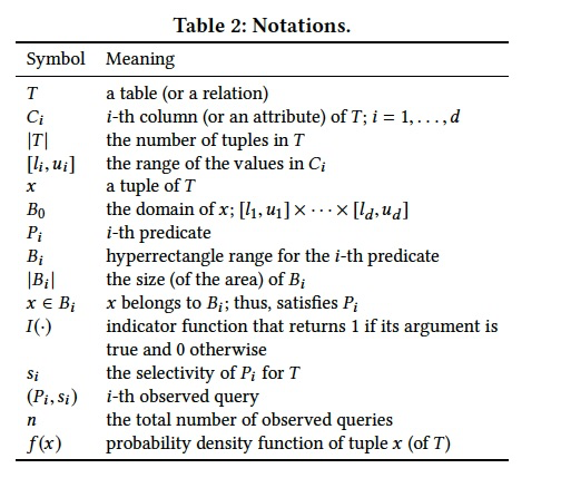
Problem Statement
Problem 1 (Query-driven Selectivity Estimation)
Consider a set of n observed queries (P1, s1), . . . , (Pn, sn) for T .
By definition, we have the following for each i = 1, . . . ,n:
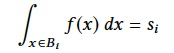
Then, our goal is to build a model of f (x) that can estimate the selectivity sn+1 of a new predicate Pn+1 .
Why not Query-driven Histograms
In this section, we briefly describe how query-driven histograms work [11, 20, 53, 67, 76, 86, 93], and then discuss their limitations, which motivate our work.
How Query-driven Histograms Work
To approximate f (x) (defined in Problem 1), query-driven histograms adjust their bucket boundaries and bucket frequencies according to the queries they observe.
Specifically, they first determine bucket boundaries (bucket creation step), and then compute their frequencies (training step), as described next.
Query-driven Histogram生成分为两个步骤,一个是Bucket Creation,一个是Training;
Bucket Creation阶段主要是,划分bucket
划分是根据query中的Predicate ranges来决定,但是这里的一个问题是,不同的query的Predicate的range一定会有overlap
参考图1,对于有overlap的地方是要做split的
1. Bucket Creation:
Query-driven histograms determine their bucket boundaries based on the given predicate’s ranges [11, 53, 76, 86, 93].
If the range of a later predicate overlaps with that of an earlier predicate,
they split the bucket(s) created for the earlier one into two or more buckets in order to ensure that the buckets do not overlap with one another.
Figure 1 shows an example of this bucket splitting operation.

Training的过程,就是计算每个bucket的frequency
早期的工作,就是直觉的在划分bucket的时候,也随便把frequency做相应的划分,这样的问题是在计算frequency时只考虑最新的query,而没有考虑其他的query
所以近期的工作都是基于最大熵原则,这是个最优化的问题,会带来较好的准确率
但是同时也会带来两个限制,buckets的数目会以指数级的增长;如果要做buckets的merge或prune就会破坏最优算法的假设
2. Training:
After creating the buckets, query-driven histograms assign frequencies to those buckets.
Earlywork [11, 67] determines bucket frequencies in the process of bucket creations.
That is, when a bucket is split into two or more, the frequency of the original bucket is also split (or adjusted),
such that it minimizes the estimation error for the latest observed query.
However, since this process does not minimize the (average) error across multiple queries, their estimates are much less accurate.
More recent work [53, 76, 86, 93] has addressed this limitation by explicitly solving an optimization problem based on the maximum entropy principle.
That is, they search for bucket frequencies that maximize the entropy of the distribution while remaining consistent with the actual selectivities observed.
Although using the maximum entropy principle will lead to highly accurate estimates, it still suffers from two key limitations.
Limitation 1: Exponential Number of Buckets
Since existing buckets may split into multiple ones for each new observed query, the number of buckets can potentially grow exponentially as the number of observed queries grows.
For example, in our experiment in Section 5.5, the number of buckets was 22,370 for 100 observed queries, and 318,936 for 300 observed queries.
Unfortunately, the number of buckets directly affects the training time.
Specifically, using iterative scaling —the optimization algorithm used by all previous work [53, 75, 76, 86, 93]—
the cost of each iteration grows linearly with the number of variables (i.e., the number of buckets).
This means that the cost of each iteration can grow exponentially with the number of observed queries.
Limitation 2: Non-trivial Bucket Merge/Pruning
Given that query-driven histograms [76, 93] quickly become infeasible due to their large number of buckets,
one might consider merging or pruning the buckets in an effort to reduce their training times.
However, merging or pruning the histogram buckets violates the assumption used by their optimization algorithms, i.e., iterative scaling.
Specifically, iterative scaling relies on the fact that a bucket is either completely included in a query’s predicate range or completely outside of it.
That is, no partial overlap is allowed. This property must hold for each of the n predicates.
However, merging some of the buckets will inevitably cause partial overlaps (between predicate and histogram buckets).
QUICKSEL: MODEL
This section presents how QuickSel models the population distribution and estimates the selectivity of a new query.
QuickSel’s model relies on a probabilistic model called a mixture model.
Uniform Mixture Model
混合模型,用一堆简单的概率密度函数的组合来表达一个复杂的概率密度函数。
而这里用到的均匀混合模型,就是用一组均匀分布密度函数,来模拟一个复杂的函数
其中,g(x)就是均匀密度函数,h(x)是权值函数,均匀密度函数在组合的时候需要一组权重值;
A mixture model is a probabilistic model that expresses a (complex) probability density function (of the population) as a combination of (simpler) probability density functions (of subpopulations).
The population distribution is the one that generates the tuple x of T.
The subpopulations are internally managed by QuickSel to best approximate f (x).
Uniform Mixture Model
QuickSel uses a type of mixture model, called the uniform mixture model .
The uniform mixture model represents a population distribution f (x) as a weighted summation of multiple uniform distributions,
gz(x) for z = 1, . . . ,m . Specifically,

where h(z) is a categorical distribution that determines the weight of the z-th subpopulation,
and gz(x) is the probability density function (which is a uniform distribution) for the zth subpopulation.
The support of h(z) is the integers ranging from 1 to m ; h(z) = wz .
The support for gz(x) is represented by a hyperrectangle Gz.
Since gz(x) is a uniform distribution, gz(x) = 1/|Gz| if x ∈ Gz and 0 otherwise. 因为是均匀分布函数,|Gz|表示这个hyperrectangle的体积,所以gz(x)任意一点,分之一
The locations of Gz and the values of wz are determined in the training stage (Section 4).
In the remainder of this section (Section 3), we assume that Gz and wz are given.
Benefit of Uniform Mixture Model
The uniform mixture model was studied early in the statistics community [27, 37];
however, recently, a more complex model called the Gaussian mixture model has received more attention [18, 84, 110]. 这里如果用高斯混合模型肯定会有更好的准确率,因为比均匀分布更符合现实,但是计算代价大幅提升
The Gaussian mixture model uses a Gaussian distribution for each subpopulation;
the smoothness of its probability density function (thus, differentiable) makes the model more appealing when gradients need to be computed.
Nevertheless, we intentionally use the uniform mixture model for QuickSel due to its computational benefit in the training process, as we describe below.
Subpopulations from Observed Queries
描述如何划分Gz边界的算法,等同于前面Query-driven Histogram的buckets creation,
这里说划分的算法和后面的training的算法是正交的,可以独立选择
划分算法,分为两种,sampling和clustering,区别就是在选择Gz center的时候是用,random还是聚类算法
We describe QuickSel’s approach to determining the boundaries of Gz for z = 1, . . . ,m.
Note that determining Gz is orthogonal to the model training process, which we describe in Section 4;
thus, even if one devises an alternative approach to creating Gz, our fast training method is still applicable.
QuickSel creates m hyperrectangular ranges (for the supports of its subpopulations) in a way that satisfies the following simple criterion:
if more predicates involve a point x, use a larger number of subpopulations for x.
Unlike query-driven histograms, QuickSel can easily pursue this goal by exploiting the property of a mixture model:
the supports of subpopulations may overlap with one another.
In short, QuickSel generates multiple points (using predicates) that represent the query workloads and create hyperrectangles that can sufficiently cover those points.
Specifically, we propose two approaches for this: a sampling-based one and a clustering-based one.
The sampling-based approach is faster; the clustering-based approach is more accurate.
Each of these is described in more detail below.
Sampling-based
This approach performs the following operations for creating Gz for z = 1, . . . ,m.
1. Within each predicate range, generate multiple random points r. 对于每个Predicate Range,都产生多个随机的抽样点
Generating a large number of random points increases the consistency;
however, QuickSel limits the number to 10 since having more than 10 points did not improve accuracy in our preliminary study.
2. Use simple random sampling to reduce the number of points to m, which serves as the centers of Gz for z = 1, . . . ,m. 从上面的点中,随机选择Gz的center点
3. The length of the i-th dimension of Gz is set to twice the average of the distances (in the same i-th dimension) to the 10 nearest-neighbor centers. 到最近的10个center点的距离的两倍作为Gz的length

Figure 2 illustrates how the subpopulations are created using both (1) highly-overlapping query workloads and (2) scattered query workloads. 这里比较高度重叠点和分散点两种情况
In both cases, QuickSel generates random points to represent the distribution of query workloads,
which is then used to create Gz (z = 1, . . . ,m ), i.e., the supports of subpopulations.
This sampling-based approach is faster, but it does not ensure the coverage of all random points r.
In contrast, the following clustering-based approach ensures that.
Clustering-based
The second approach relies on a clustering algorithm for generating hyperrectangles:
1. Do the same as the sampling-based approach.
2. Cluster r into m groups. (We used K-means++.) 差别就是这里中心点,是通过聚类算法产生
3. For each of m groups, we create the smallest hyperrectangle Gz that covers all the points belonging to the group. Gz的范围,最小的覆盖该group中的所有的point
Note that since each r belongs to a cluster and we have created a hyperrectangle that fully covers each cluster, the union of the hyperrectangles covers all r.
Our experiments primarily use the sampling-based approach due to its efficiency, but we also compare them empirically in Section 5.7.
The following section describes how to assign the weights (i.e., h(z) = wz ) of these subpopulations.
QUICKSEL: MODEL TRAINING
This section describes how to compute the weights wz of QuickSel’s subpopulations.
For training its model, QuickSel finds the model that maximizes uniformity while being consistent with the observed queries.
Training as Optimization
B0就是整个X值域空间,g0就是整体符合均匀分布
这里的L2,就是平方距离,有点类似罚项,
首先f(x)的训练目标一定是要符合观察到的query,这里同时还要求f(x)和均匀分布尽可能的接近
This section formulates an optimization problem for QuickSel’s training.
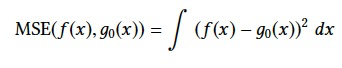
Let g0(x) be the uniform distribution with support B0; that is, g0(x) = 1/|B0| if x ∈ B0 and 0 otherwise.
QuickSel aims to find the model f (x), such that the difference between f (x) and g0(x) is minimized while being consistent with the observed queries.
There are many metrics that can measure the distance between two probability density functions f (x) and g0(x),
such as the earth mover’s distance [89], Kullback-Leibler divergence [63], the mean squared error (MSE), the Hellinger distance, and more.
Among them, QuickSel uses MSE (which is equivalent to L2 distance between two distributions)
since it enables the reduction of our originally formulated optimization problem (presented shortly; Problem 2) to a quadratic programming problem,
which can be solved efficiently by many off-the-shelf optimization libraries [1, 4, 5, 14].
Also, minimizing MSE between f (x) and g0(x) is closely related to maximizing the entropy of f (x) [53, 76, 86, 93]. See Section 6 for the explanation of this relationship.
MSE between f (x) and g0(x) is defined as follows:

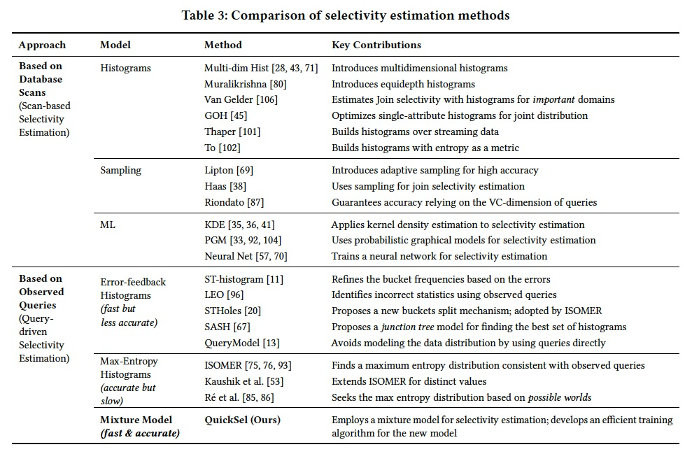
RELATEDWORK
There is extensive work on selectivity estimation due to its importance for query optimization.
Database Scan-based Estimation
As explained in Section 1,we use the term scan-based methods to refer to techniques that directly inspect the data (or part of it) for collecting their statistics.
These approaches differ from query-based methods which rely only on the actual selectivities of the observed queries.
Scan-based Histograms
These approaches approximate the joint distribution by periodically scanning the data.
There has been much work on how to efficiently express the joint distribution of multidimensional data [24, 26, 28, 34–36, 38, 40, 41, 43–45, 50, 52, 65, 69, 71, 78, 80, 87, 101, 102, 106].
There is also some work on histograms for special types of data, such as XML [10, 17, 107, 109], spatial data [49, 58–60, 68, 73, 81, 97, 99, 100, 108, 112, 113], graph [30], string [46–48, 77]; or for privacy [39, 64, 66].
Sampling
Sampling-based methods rely on a sample of data for estimating its joint distribution [38, 69, 87].
However, drawing a new random sample requires a table-scan or random retrieval of tuples, both of which are costly operations and hence, are only performed periodically.
Machine Learning Models
这里和KDE的比较,KDE和MM都是用来替代Histogram的,并且都是用一些基础函数来模拟一个概率密度函数;
他们最大的不同是,KDE需要独立同分布的samples,所以是scan-based的方法;而MM没这个限制,所以是query-based方法,跟容易实现。
KDE is a technique that translates randomly sampled data points into a distribution [91].
In the context of selectivity estimation, KDE has been used as an alternative to histograms [35, 36, 41].
The similarity between KDE and mixture models (which we employ for QuickSel) is that they both express a probability density function as a summation of some basis functions.
However, KDE and MM (mixture models) are fundamentally different.
KDE relies on independent and identically distributed samples, and hence lends itself to scan-based selectivity estimation.
In contrast, MM does not require any sampling and can thus be used in query-driven selectivity estimation (where sampling is not practical).
Similarly, probabilistic graphical models [33, 92, 104], neural networks [57, 70], and tree-based ensembles [29] have been used for selectivity estimation.
Unlike histograms, these approaches can capture column correlations more succinctly(简洁的).
However, applicability of these models for query-driven selectivity estimation has not been explored and remains unclear.
More recently, sketching [21] and probe executions [103] have been proposed, which differ from ours in that they build their models directly using the data (not query results).
Similar to histograms, using the data requires either periodic updates or higher query processing overhead.
QuickSel avoids both of these shortcomings with its query-driven MM.
Query-driven Estimation
Query-driven techniques create their histogram buckets adaptively according to the queries they observe in the workload.
These can be further categorized into two techniques based on how they compute their bucket frequencies:
error-feedback histograms and max-entropy histograms.
Error-feedback Histograms
Error-feedback histograms [11, 13, 20, 55, 56, 67] adjust bucket frequencies in consideration of the errors made by old bucket frequencies.
They differ in how they create histogram buckets according to the observed queries.
For example, STHoles [20] splits existing buckets with the predicate range of the new query.
SASH [67] uses a space-efficient multidimensional histogram, called MHIST [28], but determines its bucket frequencies with an error-feedback mechanism.
QueryModel [13] treats the observed queries themselves as conceptual histogram buckets and determines the distances among those buckets based on the similarities among the queries’ predicates.
Max-Entropy Histograms
Max-entropy histograms [53, 75, 76, 86, 93] find a maximum entropy distribution consistent with the observed queries.
Unfortunately, these methods generally suffer from the exponential growth in their number of buckets as the number of observed queries grows (as discussedin Section 2).
QuickSel avoids this problem by relying on mixture models.
Fitting Parametric Functions
Adaptive selectivity estimation [23] fits a parametric function (e.g., linear, polynomial) to the observed queries. 拟合回归的方式,但是需要有先验的知识来选择分布函数
This approach is more applicable when we know the data distribution a priori , which is not assumed by QuickSel.
Self-tuning Databases
Query-driven histograms have also been studied in the context of self-tuning databases [61, 72, 74].
IBM’s LEO [96] corrects errors in any stage of query execution based on the observed queries.
Microsoft’s AutoAdmin [12, 22] focuses on automatic physical design, self-tuning histograms, and monitoring infrastructure.
Part of this effort is ST-histogram [11] and STHoles [20] (see Table 3).
DBL [82] and IDEA [31] exploit the answers to past queries for more accurate approximate query processing.
QueryBot 5000 [72] forecasts the future queries, whereas OtterTune [105] and index [62] use machine learning for automatic physical design and building secondary indices, respectively.