Tensorflow:DCGAN生成手写数字

参考地址：https://blog.csdn.net/miracle_ma/article/details/78305991

使用DCGAN（deep convolutional GAN）：深度卷积GAN

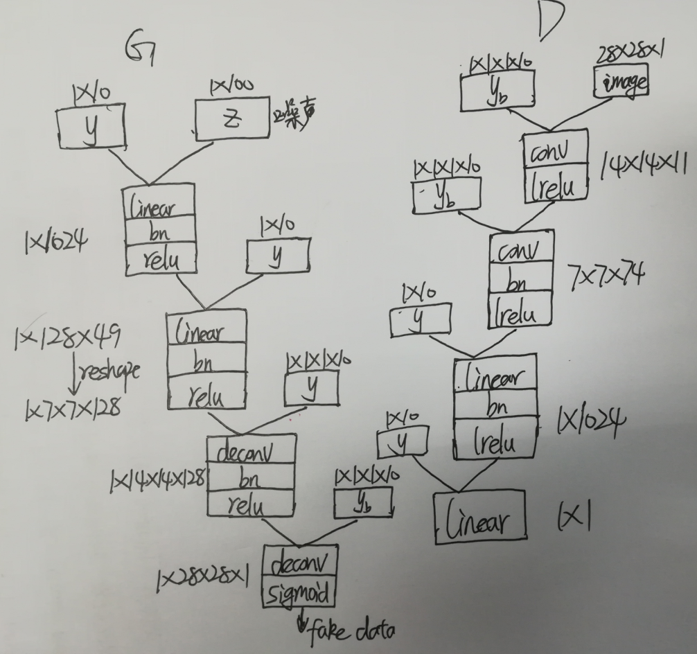
网络结构如下：

代码分成四个文件：

• 读入文件                                          read_data.py
• 配置线性层，卷积层，反卷积层     ops.py
• 构建生成器和判别器模型                model.py
• 训练模型                                          train.py

使用的layer种类有：

• conv（卷积层）
• deconv（反卷积层）
• linear（线性层）
• batch_norm（批量归一化层）
• lrelu/relu/sigmoid（非线性函数层）

一、读入文件（read_data.py）

import os
import numpy as np
import tensorflow as tf

def read_data():
    data_dir = "datamnist"
    #read training data
    fd = open(os.path.join(data_dir,"train-images.idx3-ubyte"))
    loaded = np.fromfile(file = fd, dtype = np.uint8)
    trainX = loaded[16:].reshape((60000, 28, 28, 1)).astype(np.float)

    fd = open(os.path.join(data_dir,"train-labels.idx1-ubyte"))
    loaded = np.fromfile(file = fd, dtype = np.uint8)
    trainY = loaded[8:].reshape((60000)).astype(np.float)

    #read test data
    fd = open(os.path.join(data_dir,"t10k-images.idx3-ubyte"))
    loaded = np.fromfile(file = fd, dtype = np.uint8)
    testX = loaded[16:].reshape((10000, 28, 28, 1)).astype(np.float)

    fd = open(os.path.join(data_dir,"t10k-labels.idx1-ubyte"))
    loaded = np.fromfile(file = fd, dtype = np.uint8)
    testY = loaded[8:].reshape((10000)).astype(np.float)

    # 将两个集合合并成70000大小的数据集
    X = np.concatenate((trainX, testX), axis = 0)
    y = np.concatenate((trainY, testY), axis = 0)

    print(X[:2])
    #set the random seed
    seed = 233
    np.random.seed(seed)
    np.random.shuffle(X)
    np.random.seed(seed)
    np.random.shuffle(y)

    return X/255, y

新建一个data文件夹，存放mnist数据集。读入训练集和测试集，将两个集合合并成一个70000的数据集，设置相同的随机种子，保证两个集合随机成相同的顺序。最后把X归一化到 [0, 1] 之间

二、配置线性层，卷积层，反卷积层 （ops.py）

import tensorflow as tf
from tensorflow.contrib.layers.python.layers import batch_norm as batch_norm

def linear_layer(value, output_dim, name = 'linear_connected'):
    with tf.variable_scope(name):
        try:
            # 线性层的权重
                # 名称：weights
                # shape = [int(value.get_shape()[1]), output_dim], 我们需要传入最后输出多少维，也即是output_dim的值
                # 初始化：使用标准正态截断函数 标准差是0.02
            weights = tf.get_variable('weights',
                [int(value.get_shape()[1]), output_dim],
                initializer = tf.truncated_normal_initializer(stddev = 0.02))
            # 线性层的偏置
                # 名称：biases
                # shape = [output_dim], 偏置与输出的维度相同
                # 初始化：使用常量初始化  初始化为0
            biases = tf.get_variable('biases',
                [output_dim], initializer = tf.constant_initializer(0.0))
        except ValueError:
            tf.get_variable_scope().reuse_variables()
            weights = tf.get_variable('weights',
                [int(value.get_shape()[1]), output_dim],
                initializer = tf.truncated_normal_initializer(stddev = 0.02))
            biases = tf.get_variable('biases',
                [output_dim], initializer = tf.constant_initializer(0.0))
        return tf.matmul(value, weights) + biases

def conv2d(value, output_dim, k_h = 5, k_w = 5, strides = [1,1,1,1], name = "conv2d"):
    with tf.variable_scope(name):
        try:
            # 反卷积层的权重
                # 名称：weights
                # [5, 5, 输入的维度， 输出的维度]
                # 初始化：使用标准正态截断函数 标准差是0.02
            weights = tf.get_variable('weights',
                [k_h, k_w, int(value.get_shape()[-1]), output_dim],
                initializer = tf.truncated_normal_initializer(stddev = 0.02))
            # 线性层的偏置
                # 名称：biases
                # shape = [output_shape[-1]], 偏置与输出的维度相同
                # 初始化：使用常量初始化  初始化为0
            biases = tf.get_variable('biases',
                [output_dim], initializer = tf.constant_initializer(0.0))
        except ValueError:
            tf.get_variable_scope().reuse_variables()
            weights = tf.get_variable('weights',
                [k_h, k_w, int(value.get_shape()[-1]), output_dim],
                initializer = tf.truncated_normal_initializer(stddev = 0.02))
            biases = tf.get_variable('biases',
                [output_dim], initializer = tf.constant_initializer(0.0))
        conv = tf.nn.conv2d(value, weights, strides = strides, padding = "SAME")
        conv = tf.reshape(tf.nn.bias_add(conv, biases), conv.get_shape())
        return conv

def deconv2d(value, output_shape, k_h = 5, k_w = 5, strides = [1,1,1,1], name = "deconv2d"):
    with tf.variable_scope(name):
        try:
            # 反卷积层的权重
            # filter : [height, width, output_channels, in_channels]
                # 名称：weights
                # [5, 5, 输出的维度， 输入的维度]
                # 初始化：使用标准正态截断函数 标准差是0.02
            weights = tf.get_variable('weights',
                [k_h, k_w, output_shape[-1], int(value.get_shape()[-1])],
                initializer = tf.truncated_normal_initializer(stddev = 0.02))
            # 线性层的偏置
                # 名称：biases
                # shape = [output_shape[-1]], 偏置与输出的维度相同
                # 初始化：使用常量初始化  初始化为0
            biases = tf.get_variable('biases',
                [output_shape[-1]], initializer = tf.constant_initializer(0.0))
        except ValueError:
            tf.get_variable_scope().reuse_variables()
            weights = tf.get_variable('weights',
                [k_h, k_w, output_shape[-1], int(value.get_shape()[-1])],
                initializer = tf.truncated_normal_initializer(stddev = 0.02))
            biases = tf.get_variable('biases',
                [output_shape[-1]], initializer = tf.constant_initializer(0.0))
        deconv = tf.nn.conv2d_transpose(value, weights, output_shape, strides = strides)
        deconv = tf.reshape(tf.nn.bias_add(deconv, biases), deconv.get_shape())
        return deconv

def conv_cond_concat(value, cond, name = 'concat'):
    value_shapes = value.get_shape().as_list()
    cond_shapes = cond.get_shape().as_list()

    with tf.variable_scope(name):
        return tf.concat([value, cond * tf.ones(value_shapes[0:3] + cond_shapes[3:])], 3, name = name)

# 批量归一化层
def batch_norm_layer(value, is_train = True, name = 'batch_norm'):
    with tf.variable_scope(name) as scope:
        if is_train:
            return batch_norm(value, decay = 0.9, epsilon = 1e-5, scale = True,
                                is_training = is_train, updates_collections = None, scope = scope)
        else :
            return batch_norm(value, decay = 0.9, epsilon = 1e-5, scale = True,
                            is_training = is_train, reuse = True,
                            updates_collections = None, scope = scope)

def lrelu(x, leak = 0.2, name = 'lrelu'):
    with tf.variable_scope(name):
        return tf.maximum(x, x*leak, name = name)

主要就是配置各个层的权重和参数，conv_cond_concat是为了用于卷积层计算的四维数据[batch_size, w, h, c]和约束条件y连接起来的操作，需要把两个数据的前三维转化到一样大小才能使用tf.concat(拼接函数)

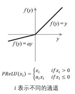
lrelu是relu的改良版。代码中a = 0.2

三、构建生成器和判别器模型（model.py）

import tensorflow as tf
from ops import *

BATCH_SIZE = 64

# 生成器模型
def generator(z, y,train = True):
    with tf.variable_scope('generator', reuse=tf.AUTO_REUSE):
        # 生成器的输入，z是 1 * 100 维的噪声
        yb = tf.reshape(y, [BATCH_SIZE, 1, 1, 10], name = 'g_yb')
        # 将噪声 z 和 y 拼接起来
        z_y = tf.concat([z,y], 1, name = 'g_z_concat_y')

        # 经过线性层，z_y 变成1024维
        linear1 = linear_layer(z_y, 1024, name = 'g_linear_layer1')
        # 先批量归一化，然后经过relu层，得 bn1
        bn1 = tf.nn.relu(batch_norm_layer(linear1, is_train = True, name = 'g_bn1'))

        # 将 bn1 与 y 拼接在一起
        bn1_y = tf.concat([bn1, y], 1 ,name = 'g_bn1_concat_y')
        # 经过线性层，变成128 * 49
        linear2 = linear_layer(bn1_y, 128*49, name = 'g_linear_layer2')
        # 先批量归一化，然后经过relu层，得 bn2
        bn2 = tf.nn.relu(batch_norm_layer(linear2, is_train = True, name = 'g_bn2'))
        # reshape成 7 * 7 * 128
        bn2_re = tf.reshape(bn2, [BATCH_SIZE, 7, 7, 128], name = 'g_bn2_reshape')

        # 将 bn2_re 与 yb 连接起来
        bn2_yb = conv_cond_concat(bn2_re, yb, name = 'g_bn2_concat_yb')
        # 经过反卷积 步长设为2，height和width 都翻倍
        deconv1 = deconv2d(bn2_yb, [BATCH_SIZE, 14, 14, 128], strides = [1, 2, 2, 1], name = 'g_deconv1')
        # 先批量归一化，然后经过relu层，得 bn3
        bn3 = tf.nn.relu(batch_norm_layer(deconv1, is_train = True, name = 'g_bn3'))

        # 将 bn2_re 与 yb 连接起来
        bn3_yb = conv_cond_concat(bn3, yb, name = 'g_bn3_concat_yb')
        # 经过反卷积 步长设为2，height和width 都翻倍
        deconv2 = deconv2d(bn3_yb, [BATCH_SIZE, 28, 28, 1], strides = [1, 2, 2, 1], name = 'g_deconv2')

        # 经过sigmoid层
        return tf.nn.sigmoid(deconv2)

# 判别器模型
def discriminator(image, y, reuse=tf.AUTO_REUSE, train = True):
    with tf.variable_scope('discriminator', reuse=tf.AUTO_REUSE):
        # 判别器有两个输入，一个是真实图片，另一个是生成的图片，都是 28 * 28
        yb = tf.reshape(y, [BATCH_SIZE, 1, 1, 10], name = 'd_yb')
        # 将 image 与 yb 连接起来
        image_yb = conv_cond_concat(image, yb, name = 'd_image_concat_yb')
        # 卷积：步长为2   14 * 14 * 11
        conv1 = conv2d(image_yb, 11, strides = [1, 2, 2, 1], name = 'd_conv1')
        # 经过 lrelu 层
        lr1 = lrelu(conv1, name = 'd_lrelu1')

        # 将 lr1 与 yb 连接起来
        lr1_yb = conv_cond_concat(lr1, yb, name = 'd_lr1_concat_yb')
        # 卷积：步长为2   7 * 7 * 74
        conv2 = conv2d(lr1_yb, 74, strides = [1, 2, 2, 1], name = 'd_conv2')
        # 批量归一化
        bn1 = batch_norm_layer(conv2, is_train = True, name = 'd_bn1')
        # 经过 lrelu 层
        lr2 = lrelu(bn1, name = 'd_lrelu2')
        lr2_re = tf.reshape(lr2, [BATCH_SIZE, -1], name = 'd_lr2_reshape')

        # 将 lr2_re 与 y 连接起来
        lr2_y = tf.concat([lr2_re, y], 1, name = 'd_lr2_concat_y')
        # 经过线性层 变成 1 * 1024
        linear1 = linear_layer(lr2_y, 1024, name = 'd_linear_layer1')
        # 批量归一化
        bn2 = batch_norm_layer(linear1, is_train = True, name = 'd_bn2')
        # 经过 lrelu 层
        lr3 = lrelu(bn2, name = 'd_lrelu3')

        lr3_y = tf.concat([lr3, y], 1, name = 'd_lr3_concat_y')
        linear2 = linear_layer(lr3_y, 1, name = 'd_linear_layer2')

        return linear2

def sampler(z, y, train = True):
    tf.get_variable_scope().reuse_variables()
    return generator(z, y, train = train)

按照模型图实现生成器G，返回时用到了sigmoid，将输出值规范到（0， 1）与前面输入图像的范围一致。

判别器D：

1、 设置reuse变量（变量重复使用）。判别器有两个输入。对于同一个D，先喂给它real data（真实的图像），然后喂给它fake data（生成器生成的假图像）。在一次train_step里涉及到了两次D变量的重复使用，所以需要设置变量共享。

2、返回值没有使用sigmoid，因为训练中使用了sigmoid_cross_entropy_with_logits来计算loss

四、训练模型

import scipy.misc
import numpy as np
import tensorflow as tf
import os
from read_data import *
from ops import *
from model import *

BATCH_SIZE = 64

# 保存图片，将图片拼接在一起
def save_images(images, size, path):
    img = (images + 1.0)/2.0
    h, w = img.shape[1], img.shape[2]

    merge_img = np.zeros((h * size[0], w * size[1], 3))

    for idx, image in enumerate(images):
        i = idx % size[1]
        j = idx // size[1]
        merge_img[j*h:j*h+h,i*w:i*w+w,:] = image

    return scipy.misc.imsave(path, merge_img)

def train():

    #read data
    X, Y = read_data()

    #global_step to record the step of training
    global_step = tf.Variable(0, name = 'global_step', trainable = True)

    # 创建placeholder
    y = tf.placeholder(tf.int32, [BATCH_SIZE], name = 'y')
    _y = tf.one_hot(y, depth = 10, on_value=None, off_value=None, axis=None, dtype=None, name='one_hot')
    z = tf.placeholder(tf.float32, [BATCH_SIZE, 100], name = 'z')
    images = tf.placeholder(tf.float32, [BATCH_SIZE, 28, 28, 1], name = 'images')

    # 用噪声生成图片
    G = generator(z, _y)
    # 用真实图片训练判别器
    D = discriminator(images, _y)
    # 用生成的加图片G训练判别器
    _D = discriminator(G, _y)

    # 计算损失值，使用 sigmoid_cross_entropy_with_logits
    # 真实图片在判别器里产生的loss，我们希望真实图片在判别器里的label趋向于1
    d_loss_real = tf.reduce_mean(tf.nn.sigmoid_cross_entropy_with_logits(logits = D, labels = tf.ones_like(D)))

    # 假图片在判别器里产生的loss，我们希望假图片在判别器里的label趋向于0
    d_loss_fake = tf.reduce_mean(tf.nn.sigmoid_cross_entropy_with_logits(logits = _D, labels = tf.zeros_like(_D)))

    # 假图片在判别器上的结果，我们希望它以假乱真，希望它尽可能接近于1
    g_loss = tf.reduce_mean(tf.nn.sigmoid_cross_entropy_with_logits(logits = _D, labels = tf.ones_like(_D)))
    
    # 判别器的总 loss
    d_loss = d_loss_real + d_loss_fake

    t_vars = tf.trainable_variables()
    d_vars = [var for var in t_vars if 'd_' in var.name]
    g_vars = [var for var in t_vars if 'g_' in var.name]

    with tf.variable_scope(tf.get_variable_scope(), reuse = False):
        # 优化判别器的 loss
        d_optim = tf.train.AdamOptimizer(0.0002, beta1 = 0.5).minimize(d_loss, var_list = d_vars, global_step = global_step)
        # 优化生成器的 loss
        g_optim = tf.train.AdamOptimizer(0.0002, beta2 = 0.5).minimize(g_loss, var_list = g_vars, global_step = global_step)

    #tensorborad
    train_dir = 'logs'
    z_sum = tf.summary.histogram("z",z)
    d_sum = tf.summary.histogram("d",D)
    d__sum = tf.summary.histogram("d_",_D)
    g_sum = tf.summary.histogram("g", G)

    d_loss_real_sum = tf.summary.scalar("d_loss_real", d_loss_real)
    d_loss_fake_sum = tf.summary.scalar("d_loss_fake", d_loss_fake)
    g_loss_sum = tf.summary.scalar("g_loss", g_loss)
    d_loss_sum = tf.summary.scalar("d_loss", d_loss)

    g_sum = tf.summary.merge([z_sum, d__sum, g_sum, d_loss_fake_sum, g_loss_sum])
    d_sum = tf.summary.merge([z_sum, d_sum, d_loss_real_sum, d_loss_sum])

    #initial
    init = tf.global_variables_initializer()
    sess = tf.InteractiveSession()
    writer = tf.summary.FileWriter(train_dir, sess.graph)

    #save
    saver = tf.train.Saver()
    # 保存模型
    check_path = "./save/model.ckpt"

    #sample
    sample_z = np.random.uniform(-1, 1, size = (BATCH_SIZE, 100))
    sample_labels = Y[0:BATCH_SIZE]

    #make sample
    sample = sampler(z, _y)

    #run
    sess.run(init)
    #saver.restore(sess.check_path)

    #train
    for epoch in range(10):
        batch_idx = int(70000/64)
        for idx in range(batch_idx):
            batch_images = X[idx*64:(idx+1)*64]
            batch_labels = Y[idx*64:(idx+1)*64]
            batch_z = np.random.uniform(-1, 1, size = (BATCH_SIZE, 100))

            _, summary_str = sess.run([d_optim, d_sum],
                                    feed_dict = {images: batch_images,
                                                 z: batch_z,
                                                 y: batch_labels})
            writer.add_summary(summary_str, idx+1)

            _, summary_str = sess.run([g_optim, g_sum],
                                    feed_dict = {images: batch_images,
                                                 z: batch_z,
                                                 y: batch_labels})
            writer.add_summary(summary_str, idx+1)

            d_loss1 = d_loss_fake.eval({z: batch_z, y: batch_labels})
            d_loss2 = d_loss_real.eval({images: batch_images, y:batch_labels})
            D_loss = d_loss1 + d_loss2
            G_loss = g_loss.eval({z: batch_z, y: batch_labels})

            #every 20 batch output loss
            if idx % 20 == 0:
                print("Epoch: %d [%4d/%4d] d_loss: %.8f, g_loss: %.8f" % (epoch, idx, batch_idx, D_loss, G_loss))

            #every 100 batch save a picture
            if idx % 100 == 0:
                sap = sess.run(sample, feed_dict = {z: sample_z, y: sample_labels})
                samples_path = './sample/'
                save_images(sap, [8,8], samples_path+'test_%d_epoch_%d.png' % (epoch, idx))

            #every 500 batch save model
            if idx % 500 == 0:
                saver.save(sess, check_path, global_step = idx + 1)
    sess.close()

if __name__ == '__main__':
    train()

模型的训练顺序是先generator生成fake data，然后real data喂给D训练，再把fake data喂给D训练

分别计算生成器和判别器的loss，其中判别器的loss = real loss + fake loss

一个batch中，训练一次D训练一次G。按理说应该训练k次D，训练一次G（为了方便就没有这么做了）

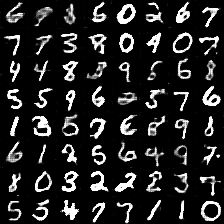
生成的效果图如下：