sklearn常见分类器的效果比较

sklearn 是 python 下的机器学习库。

scikit-learn的目的是作为一个“黑盒”来工作，即使用户不了解实现也能产生很好的结果。

其功能非常强大，当然也有很多不足的地方，就比如说神经网络就只有一个RBM（不是人民币哈）。但是，不管怎样，首荐！！

这个例子比较了几种分类器的效果，并直观的显示之

import numpy as np
import matplotlib.pyplot as plt
from matplotlib.colors import ListedColormap
#from sklearn.model_selection import train_test_split #废弃！！
from sklearn.cross_validation import train_test_split
from sklearn.preprocessing import StandardScaler
from sklearn.datasets import make_moons, make_circles, make_classification
from sklearn.neural_network import BernoulliRBM
from sklearn.neighbors import KNeighborsClassifier
from sklearn.svm import SVC
from sklearn.gaussian_process import GaussianProcess
from sklearn.tree import DecisionTreeClassifier
from sklearn.ensemble import RandomForestClassifier, AdaBoostClassifier
from sklearn.naive_bayes import GaussianNB
from sklearn.discriminant_analysis import QuadraticDiscriminantAnalysis

h = .02  # step size in the mesh

names = ["Nearest Neighbors", "Linear SVM", "RBF SVM",
         "Decision Tree", "Random Forest", "AdaBoost",
         "Naive Bayes", "QDA", "Gaussian Process","Neural Net", ]

classifiers = [
    KNeighborsClassifier(3),
    SVC(kernel="linear", C=0.025),
    SVC(gamma=2, C=1),
    DecisionTreeClassifier(max_depth=5),
    RandomForestClassifier(max_depth=5, n_estimators=10, max_features=1),
    AdaBoostClassifier(),
    GaussianNB(),
    QuadraticDiscriminantAnalysis(),
    #GaussianProcess(),
    #BernoulliRBM(),
    ]

X, y = make_classification(n_features=2, n_redundant=0, n_informative=2,
                           random_state=1, n_clusters_per_class=1)
rng = np.random.RandomState(2)
X += 2 * rng.uniform(size=X.shape)
linearly_separable = (X, y)

datasets = [make_moons(noise=0.3, random_state=0),
            make_circles(noise=0.2, factor=0.5, random_state=1),
            linearly_separable
            ]

figure = plt.figure(figsize=(27, 9))
i = 1
# iterate over datasets
for ds_cnt, ds in enumerate(datasets):
    # preprocess dataset, split into training and test part
    X, y = ds
    X = StandardScaler().fit_transform(X)
    X_train, X_test, y_train, y_test = 
        train_test_split(X, y, test_size=.4, random_state=42)

    x_min, x_max = X[:, 0].min() - .5, X[:, 0].max() + .5
    y_min, y_max = X[:, 1].min() - .5, X[:, 1].max() + .5
    xx, yy = np.meshgrid(np.arange(x_min, x_max, h),
                         np.arange(y_min, y_max, h))

    # just plot the dataset first
    cm = plt.cm.RdBu
    cm_bright = ListedColormap(['#FF0000', '#0000FF'])
    ax = plt.subplot(len(datasets), len(classifiers) + 1, i)
    if ds_cnt == 0:
        ax.set_title("Input data")
    # Plot the training points
    ax.scatter(X_train[:, 0], X_train[:, 1], c=y_train, cmap=cm_bright)
    # and testing points
    ax.scatter(X_test[:, 0], X_test[:, 1], c=y_test, cmap=cm_bright, alpha=0.6)
    ax.set_xlim(xx.min(), xx.max())
    ax.set_ylim(yy.min(), yy.max())
    ax.set_xticks(())
    ax.set_yticks(())
    i += 1

    # iterate over classifiers
    for name, clf in zip(names, classifiers):
        ax = plt.subplot(len(datasets), len(classifiers) + 1, i)
        clf.fit(X_train, y_train)
        score = clf.score(X_test, y_test)

        # Plot the decision boundary. For that, we will assign a color to each
        # point in the mesh [x_min, m_max]x[y_min, y_max].
        if hasattr(clf, "decision_function"):
            Z = clf.decision_function(np.c_[xx.ravel(), yy.ravel()])
        else:
            Z = clf.predict_proba(np.c_[xx.ravel(), yy.ravel()])[:, 1]

        # Put the result into a color plot
        Z = Z.reshape(xx.shape)
        ax.contourf(xx, yy, Z, cmap=cm, alpha=.8)

        # Plot also the training points
        ax.scatter(X_train[:, 0], X_train[:, 1], c=y_train, cmap=cm_bright)
        # and testing points
        ax.scatter(X_test[:, 0], X_test[:, 1], c=y_test, cmap=cm_bright,
                   alpha=0.6)

        ax.set_xlim(xx.min(), xx.max())
        ax.set_ylim(yy.min(), yy.max())
        ax.set_xticks(())
        ax.set_yticks(())
        if ds_cnt == 0:
            ax.set_title(name)
        ax.text(xx.max() - .3, yy.min() + .3, ('%.2f' % score).lstrip('0'),
                size=15, horizontalalignment='right')
        i += 1

plt.tight_layout()
plt.show()

效果图：

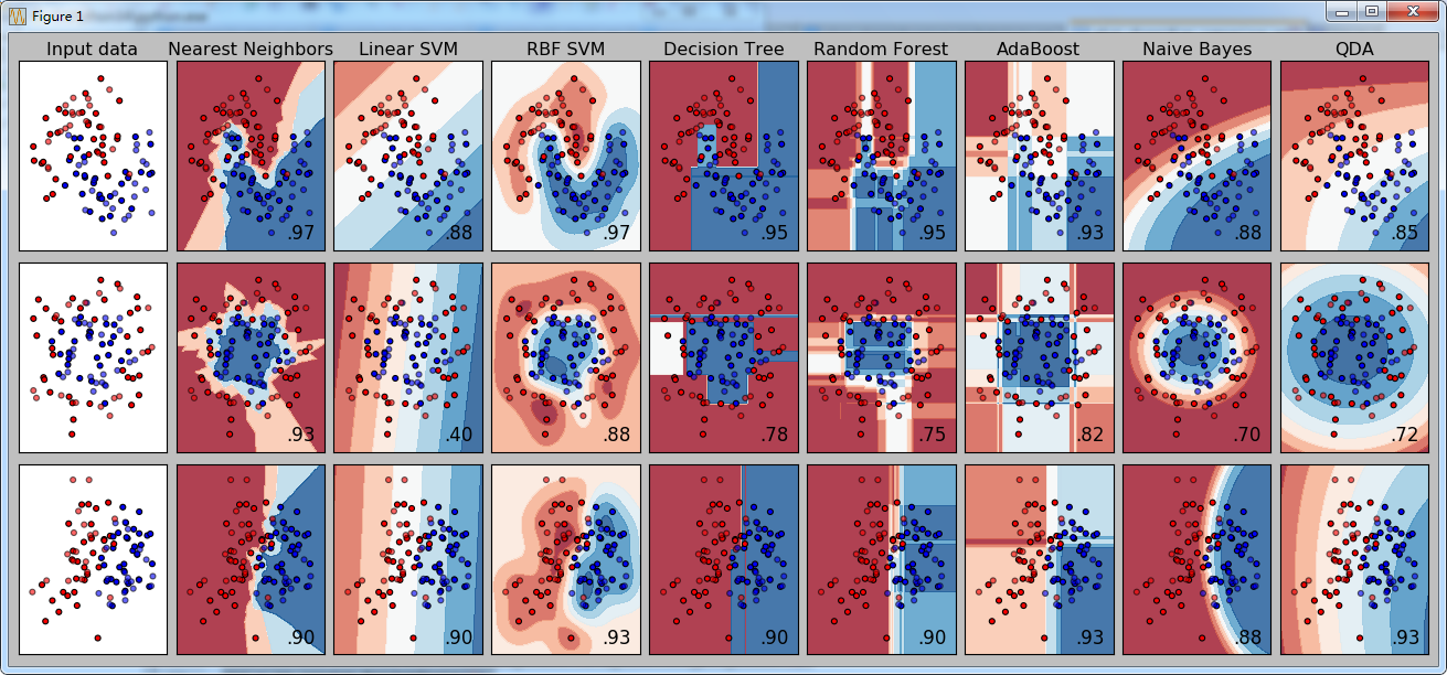
说明：

1.原始数据（三组）

2.分类器名称（八个）

3.对应的成绩 (score)