Univariate plotting with pandas


import pandas as pd
reviews = pd.read_csv("../input/wine-reviews/winemag-data_first150k.csv", index_col=0)
reviews.head(3)

//bar
reviews['province'].value_counts().head(10).plot.bar()
(reviews['province'].value_counts().head(10) / len(reviews)).plot.bar()
reviews['points'].value_counts().sort_index().plot.bar()

//line chart
reviews['points'].value_counts().sort_index().plot.line()

//area chart
reviews['points'].value_counts().sort_index().plot.area()

//histograms
reviews[reviews['price'] < 200]['price'].plot.hist()
reviews['price'].plot.hist()
reviews[reviews['price'] > 1500]

//pie chart
reviews['province'].value_counts().head(10).plot.pie()
Bivariate plotting with pandas
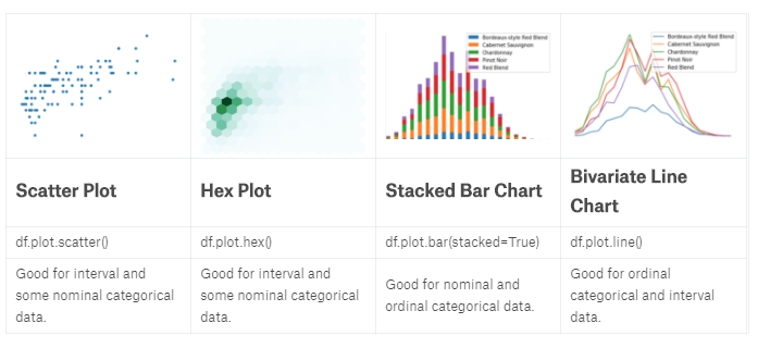
import pandas as pd
reviews = pd.read_csv("../input/wine-reviews/winemag-data_first150k.csv", index_col=0)
reviews.head()

//Scatter plot
reviews[reviews['price'] < 100].sample(100).plot.scatter(x='price', y='points')

//hexplot 数据相关性
reviews[reviews['price'] < 100].plot.hexbin(x='price', y='points', gridsize=15)

//stackplot 数据堆叠
wine_counts.plot.bar(stacked=True)
wine_counts.plot.area()

//Bivariate line chart 线集成
wine_counts.plot.line()
Plotting with seaborn
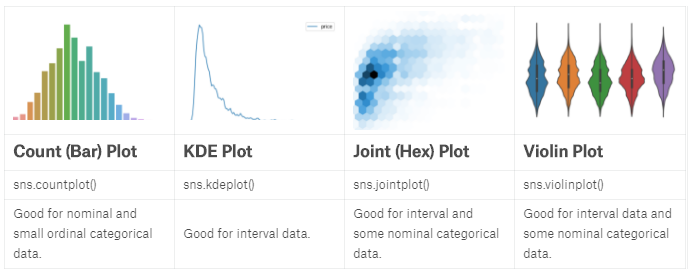
import pandas as pd
reviews = pd.read_csv("../input/wine-reviews/winemag-data_first150k.csv", index_col=0)
import seaborn as sns

//Countplot
sns.countplot(reviews['points'])

//KDE Plot 平滑去噪
sns.kdeplot(reviews.query('price < 200').price)
//对比线图
reviews[reviews['price'] < 200]['price'].value_counts().sort_index().plot.line()
//二维ked
sns.kdeplot(reviews[reviews['price'] < 200].loc[:, ['price', 'points']].dropna().sample(5000))

//Distplot
sns.distplot(reviews['points'], bins=10, kde=False)

//jointplot
sns.jointplot(x='price', y='points', data=reviews[reviews['price'] < 100])
sns.jointplot(x='price', y='points', data=reviews[reviews['price'] < 100], kind='hex', gridsize=20)


//Boxplot and violin plot   25%-75%,中线
df = reviews[reviews.variety.isin(reviews.variety.value_counts().head(5).index)]

sns.boxplot(
    x='variety',
    y='points',
    data=df
)
Faceting with seaborn
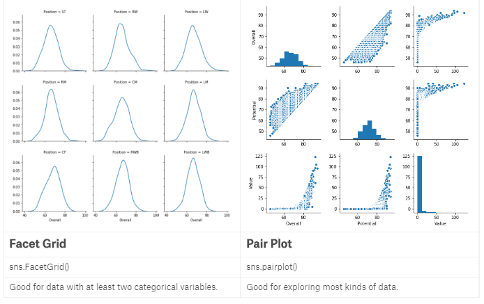
import pandas as pd
pd.set_option('max_columns', None)
df = pd.read_csv("../input/fifa-18-demo-player-dataset/CompleteDataset.csv", index_col=0)

import re
import numpy as np
import seaborn as sns

footballers = df.copy()
footballers['Unit'] = df['Value'].str[-1]
footballers['Value (M)'] = np.where(footballers['Unit'] == '0', 0,
                                    footballers['Value'].str[1:-1].replace(r'[a-zA-Z]',''))
footballers['Value (M)'] = footballers['Value (M)'].astype(float)
footballers['Value (M)'] = np.where(footballers['Unit'] == 'M',
                                    footballers['Value (M)'],
                                    footballers['Value (M)']/1000)
footballers = footballers.assign(Value=footballers['Value (M)'],
                                 Position=footballers['Preferred Positions'].str.split().str[0])


//The FacetGrid
df = footballers[footballers['Position'].isin(['ST', 'GK'])]
g = sns.FacetGrid(df, col="Position")
g.map(sns.kdeplot, "Overall")


df = footballers
g = sns.FacetGrid(df, col="Position", col_wrap=6)//,每行6列
g.map(sns.kdeplot, "Overall")


df = footballers[footballers['Position'].isin(['ST', 'GK'])]
df = df[df['Club'].isin(['Real Madrid CF', 'FC Barcelona', 'Atlético Madrid'])]
g = sns.FacetGrid(df, row="Position", col="Club",
                  row_order=['GK', 'ST'],
                  col_order=['Atlético Madrid', 'FC Barcelona', 'Real Madrid CF'])
g.map(sns.violinplot, "Overall") //violin图


//Pairplot 数据分析第一步
sns.pairplot(footballers[['Overall', 'Potential', 'Value']])
Multivariate plotting
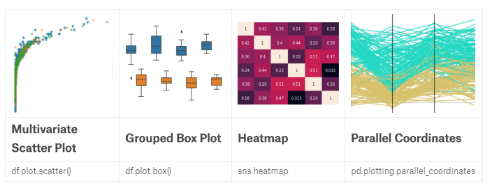
import pandas as pd
pd.set_option('max_columns', None)
df = pd.read_csv("../input/fifa-18-demo-player-dataset/CompleteDataset.csv", index_col=0)

import re
import numpy as np

footballers = df.copy()
footballers['Unit'] = df['Value'].str[-1]
footballers['Value (M)'] = np.where(footballers['Unit'] == '0', 0,
                                    footballers['Value'].str[1:-1].replace(r'[a-zA-Z]',''))
footballers['Value (M)'] = footballers['Value (M)'].astype(float)
footballers['Value (M)'] = np.where(footballers['Unit'] == 'M',
                                    footballers['Value (M)'],
                                    footballers['Value (M)']/1000)
footballers = footballers.assign(Value=footballers['Value (M)'],
                                 Position=footballers['Preferred Positions'].str.split().str[0])


//Multivariate scatter plots
import seaborn as sns
sns.lmplot(x='Value', y='Overall', hue='Position',
           data=footballers.loc[footballers['Position'].isin(['ST', 'RW', 'LW'])],
           fit_reg=False)


sns.lmplot(x='Value', y='Overall', markers=['o', 'x', '*'], hue='Position',
           data=footballers.loc[footballers['Position'].isin(['ST', 'RW', 'LW'])],
           fit_reg=False
          )

//Grouped box plot 分组的优势
f = (footballers
         .loc[footballers['Position'].isin(['ST', 'GK'])]
         .loc[:, ['Value', 'Overall', 'Aggression', 'Position']]
    )
f = f[f["Overall"] >= 80]
f = f[f["Overall"] < 85]
f['Aggression'] = f['Aggression'].astype(float)
sns.boxplot(x="Overall", y="Aggression", hue='Position', data=f)


//Heatmap
f = (
    footballers.loc[:, ['Acceleration', 'Aggression', 'Agility', 'Balance', 'Ball control']]
        .applymap(lambda v: int(v) if str.isdecimal(v) else np.nan)
        .dropna()
).corr()
sns.heatmap(f, annot=True)


//Parallel Coordinates
from pandas.plotting import parallel_coordinates

f = (
    footballers.iloc[:, 12:17]
        .loc[footballers['Position'].isin(['ST', 'GK'])]
        .applymap(lambda v: int(v) if str.isdecimal(v) else np.nan)
        .dropna()
)
f['Position'] = footballers['Position']
f = f.sample(200)
parallel_coordinates(f, 'Position')
plotly
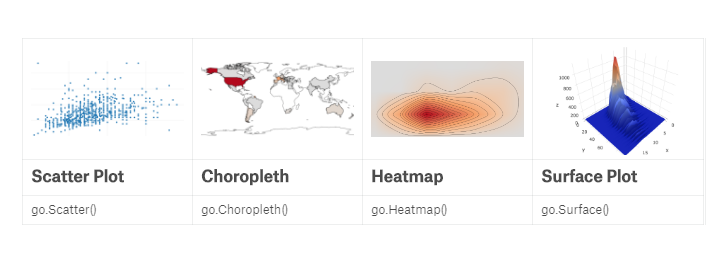
import pandas as pd
reviews = pd.read_csv("../input/wine-reviews/winemag-data-130k-v2.csv", index_col=0)
reviews.head()

from plotly.offline import init_notebook_mode, iplot
init_notebook_mode(connected=True)  #离线注入笔记本模式

import plotly.graph_objs as go
iplot([go.Scatter(x=reviews.head(1000)['points'], y=reviews.head(1000)['price'], mode='markers')])

iplot([go.Histogram2dContour(x=reviews.head(500)['points'],
                             y=reviews.head(500)['price'],
                             contours=go.Contours(coloring='heatmap')),
       go.Scatter(x=reviews.head(1000)['points'], y=reviews.head(1000)['price'], mode='markers')])


#surface图
df = reviews.assign(n=0).groupby(['points', 'price'])['n'].count().reset_index()  #先point分组再price分,再添加的‘n’列上执行计数,最后对首列的index重新排序
df = df[df["price"] < 100]
v = df.pivot(index='price', columns='points', values='n').fillna(0).values.tolist() #重塑数组后用0填充NAN值,再把values列变成list
iplot([go.Surface(z=v)])


#地理图
df = reviews['country'].replace("US", "United States").value_counts()

iplot([go.Choropleth(
    locationmode='country names',
    locations=df.index.values,
    text=df.index,
    z=df.values
)])