Spark2.0机器学习系列之6：GBDT（梯度提升决策树）、GBDT与随机森林差异、参数调试及Scikit代码分析

概念梳理

GBDT的别称

　GBDT(Gradient Boost Decision Tree),梯度提升决策树。 
    GBDT这个算法还有一些其他的名字，比如说MART(Multiple Additive Regression Tree)，GBRT(Gradient Boost Regression Tree)，Tree Net等，其实它们都是一个东西（参考自wikipedia – Gradient Boosting)，发明者是Friedman。 
研究GBDT一定要看看Friedman的paper《Greedy Function Approximation: A Gradient Boosting Machine》，里面论述和公式推导更为系统。

什么是梯度提升算法？

　　GB（Gradient Boosting）梯度提升算法 
　　GB其实是一个算法框架，即可以将已有的分类或回归算法放入其中，得到一个性能很强大的算法。 
　　GB这个框架中可以放入很多不同的算法。 
　　GB总共需要进行M次迭代，每次迭代产生一个模型，我们需要让每次迭代生成的模型对训练集的损失函数最小，而如何让损失函数越来越小呢？我们采用梯度下降的方法，在每次迭代时通过向损失函数的负梯度方向移动来使得损失函数越来越小，这样我们就可以得到越来越精确的模型。 

梯度下降算法在机器学习中会经常遇到，这里给一幅图片就好理解了： 

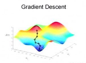
图片说明：将参数θ按照梯度下降的方向进行调整，就会使得代价函数J(θ)往更低的方向进行变化，如图所示，算法的结束将是在θ下降到无法继续下降为止。黑线就是代价（错误）下降的轨迹，始终是按照梯度方向下降的，也是下降最快的方向。 
图片来源： 
http://www.cnblogs.com/LeftNotEasy/archive/2010/12/05/mathmatic_in_machine_learning_1_regression_and_gradient_descent.html 
更详细的内容可以参考原博客。

原始Boosting算法与Gradient Boosting的区别

　　同样都是提升算法，原始Boosting算法与Gradient Boosting是有很本质区别的。 
　　原始的Boost算法是在算法开始的时候，为每一个样本赋上一个权重值，初始的时候，大家都是一样重要的。在每一步训练中得到的模型，会使得数据点的估计有对有错，我们就在每一步结束后，增加分错的点的权重，减少分对的点的权重，这样使得某些点如果老是被分错，那么就会被“严重关注”，也就被赋上一个很高的权重。然后等进行了N次迭代（由用户指定），将会得到N个简单的分类器（basic learner），然后我们将它们组合起来（比如说可以对它们进行加权、或者让它们进行投票等），得到一个最终的模型。

而Gradient Boost与传统的Boost的区别是，每一次的计算是为了减少上一次的残差(residual)，而为了消除残差，我们可以在残差减少的梯度(Gradient)方向上建立一个新的模型。所以说，在Gradient Boost中，每个新的模型的简历是为了使得之前模型的残差往梯度方向减少，与传统Boost对正确、错误的样本进行加权有着很大的区别。 
　　在GB算法框架中放入决策树，就是GBDT了。 

GBDT的两个版本

参考文章：http://blog.csdn.net/kunlong0909/article/details/17587101

（1）残差版本 
　    残差其实就是真实值和预测值之间的差值，在学习的过程中，首先学习一颗回归树，然后将“真实值-预测值”得到残差，再把残差作为一个学习目标，学习下一棵回归树，依次类推，直到残差小于某个接近0的阀值或回归树数目达到某一阀值。其核心思想是每轮通过拟合残差来降低损失函数。 
　　总的来说，第一棵树是正常的，之后所有的树的决策全是由残差来决定。 
首先给出一个简单的例子： 
如果不明白图片是什么意思，请参考： 
http://blog.csdn.net/w28971023/article/details/8240756 
 
　　可以看到第二棵数的输入是对第一棵树预测结果与实际结果的残差。因此很容易发现GBDT算法有这样一些重要的特性,会对后面Spark实际编程时参数设置（调试）有一些指导作用（后面还会详细说）。 
　　GBDT是通过迭代不断使误差减小的过程，后一棵树对前一棵树的残差进行预测，这和随机森林平行的用多棵树同时预测完全不一样。因此对树结构（如MaxDepth），运算时间，预测结果，泛化能力都和随机森林不一样。（Spark coding时再详细对比分析）

　　算法： 
　　 
（2）梯度版本 
　　与残差版本把GBDT说成一个残差迭代树，认为每一棵回归树都在学习前N-1棵树的残差不同，Gradient版本把GBDT说成一个梯度迭代树，使用梯度下降法求解，认为每一棵回归树在学习前N-1棵树的梯度下降值。总的来说两者相同之处在于，都是迭代回归树，都是累加每颗树结果作为最终结果（Multiple Additive Regression Tree)，每棵树都在学习前N-1棵树尚存的不足，从总体流程和输入输出上两者是没有区别的； 
　　两者的不同主要在于每步迭代时，是否使用Gradient作为求解方法。前者不用Gradient而是用残差—-残差是全局最优值，Gradient是局部最优方向*步长，即前者每一步都在试图让结果变成最好，后者则每步试图让结果更好一点。 
　　两者优缺点。看起来前者更科学一点–有绝对最优方向不学，为什么舍近求远去估计一个局部最优方向呢？原因在于灵活性。前者最大问题是，由于它依赖残差，cost function一般固定为反映残差的均方差，因此很难处理纯回归问题之外的问题。而后者求解方法为梯度下降，只要可求导的cost function都可以使用。 
　　算法如下： 
　　可参考http://blog.csdn.net/starzhou/article/details/51648219 
　　其实这些算法都来自Friedman的论文，想要深度研究该算法的原理，最好阅读原文自己推导一遍。 
　　 

前向分步算法(forward stagewise algorithm)

　　可以看出GBDT是一种前向分步算法。 
　　更普遍的，前向分步算法有两种形式，前一种是更新模型，是一种是加法模型： 
 
　　通俗理解就是：向前一步一步的走，逐渐逼近想要的结果。当然走的快慢，也是可以再增加一个控制参数，一个叫学习率的参数来控制（见下面正则化部分）。 

正则化(学习率）

Shrinkage 
proposed a simple regularization strategy that scales the contribution of each weak learner by a factor : 
 
The parameter : is also called the learning rate because it scales the step length the the gradient descent procedure; it can be set via the learning_rate parameter.

　　学习率和正则化怎么在一起了？通俗理解就是：每次走很小的一步逐渐逼近的效果，要比每次迈一大步很快逼近结果的方式更容易避免过拟合。

Spark2.0中GBDT

GBDT的优点

　　GBDT和随机森林一样，都具备决策树的一些优点： 
　　(1)可以处理类别特征和连续特征； 
　　(2)不需要对数据进行标准化预处理； 
　　(3)可以分析特征之间的相互影响 
　　值得注意的是，Spark中的GBDT目前还不能处理多分类问题，仅可以用于二分类和回归问题。（Spark随机森林可以处理多分类问题）　

　　Gradient-Boosted Trees (GBTs) are ensembles of decision trees. GBTs iteratively train decision trees in order to minimize a loss function. Like decision trees, GBTs handle categorical features, do not require feature scaling, and are able to capture non-linearities and feature interactions.

　　spark.mllib supports GBTs for binary classification and for regression, using both continuous and categorical features. spark.mllib implements GBTs using the existing decision tree implementation. Please see the decision tree guide for more information on trees.

　　Note: GBTs do not yet support multiclass classification. For multiclass problems, please use decision trees or Random Forests.

GBDT与随机森林应用时的对比

　　GBDT和随机森林虽然都是决策树的组合算法，但是两者的训练过程还是很不相同的。 
　　GBDT训练是每次一棵，一棵接着一棵（串行），因此与随机森林并行计算多棵树相比起来，会需要更长的训练时间。 
　　在GBDT中，相对于随机森林而言（随机森林中的树可以不做很多的剪枝），一般会选择更浅（depth更小）的树，这样运算时间会减少。 
　　随机森林更不容易过拟合，而且森林中包含越多的树似乎越不会出现过拟合。用统计学的语言来讲，就是说越多的树包含进来，会降低预测结果的方差（多次预测结果会更加稳定）。但是GBDT则恰好相反，包含预测的树（即迭代的次数越多），反而会更倾向于过拟合，用统计学的语言来将，就是GBDT迭代次数的增加减少的是偏差（预测结果和训练数据label之间的差异）。（偏差和方差这两个概念是不同的概念，见后面的图） 
　　随机森林参数相对更容易调试一些，这是由于随着所包含的决策树的个数增加，其预测效果一般是单调的向好的方向变。而GBDT则不同，一开始预测表现会随着树的数目增大而变好，但是到一定程度之后，反而会随着树的数目增加而变差。 
　　总而言之，这两种算法都还是非常有效的算法，如何选择取决于实际的数据。

   Gradient-Boosted Trees vs. Random Forests 
　　Both Gradient-Boosted Trees (GBTs) and Random Forests are algorithms for learning ensembles of trees, but the training processes are different. There are several practical trade-offs:

　　GBTs train one tree at a time, so they can take longer to train than random forests. Random Forests can train multiple trees in parallel.

　　On the other hand, it is often reasonable to use smaller (shallower) trees with GBTs than with Random Forests, and training smaller trees takes less time.

　　Random Forests can be less prone to overfitting. Training more trees in a Random Forest reduces the likelihood of overfitting, but training more trees with GBTs increases the likelihood of overfitting. (In statistical language, Random Forests reduce variance by using more trees, whereas GBTs reduce bias by using more trees.)

　　Random Forests can be easier to tune since performance improves monotonically with the number of trees (whereas performance can start to decrease for GBTs if the number of trees grows too large).

　　In short, both algorithms can be effective, and the choice should be based on the particular dataset.

偏差和方差的区别： 
　　偏差：描述的是预测值（估计值）的期望与真实值之间的差距。偏差越大，越偏离真实数据，如下图第二行所示。 
　　方差：描述的是预测值的变化范围，离散程度，也就是离其期望值的距离。方差越大，数据的分布越分散，如下图右列所示。 

关键参数

　　有三个关键参数需要仔细分析：loss，numIterations，learningRate。可以通过下面的方式设置

//定义GBTClassifier，注意在Spark中输出（预测列）都有默认的设置，可以不自己设置
GBTClassifier gbtClassifier=new GBTClassifier()
                            .setLabelCol("indexedLabel")//输入label
                            .setFeaturesCol("indexedFeatures")//输入features vector
                            .setMaxIter(MaxIter)//最大迭代次数
                            .setImpurity("entropy")//or "gini"
                            .setMaxDepth(3)//决策树的深度
                            .setStepSize(0.3)//范围是(0, 1]
                            .setSeed(1234); //可以设一个随机数种子点

loss（损失函数的类型）

　　Spark中已经实现的损失函数类型有以下三种，注意每一种都只适合一类问题，要么是回归，要么是分类。 
　　分类只可选择 Log Loss，回归问题可选择平方误差和绝对值误差。分别又称为L2损失和L1损失。绝对值误差（L1损失）在处理带有离群值的数据时比L2损失更加具有鲁棒性。 

numIterations（迭代次数）

　　GBDT迭代次数，每一次迭代将产生一棵树，因此numIterations也是算法中所包含的树的数目。增加numIterations会提高训练集数据预测准确率（注意是训练集数据上的准确率哦）。但是相应的会增加训练的时间。如何选择合适的参数防止过拟合，一定需要做验证。将数据分为两份，一份是训练集，一份是验证集。 
　　随着迭代次数的增加，一开始在验证集上预测误差会减小，迭代次数增大到一定程度后误差反而会增加，那么通过准确度vs.迭代次数曲线可以选择最合适的numIterations。

learningRate（学习率）

　　这个参数一般不需要调试，如果发现算法面对某个数据集，变现得极其不稳定，那么就要减小学习率再试一下，一般会有改善（稳定性变好）。小的学习率（步长）肯定会增加训练的时间。

　(1) loss: See the section above for information on losses and their applicability to tasks (classification vs. regression). Different losses can give significantly different results, depending on the dataset. 
　　(2) numIterations: This sets the number of trees in the ensemble. Each iteration produces one tree. Increasing this number makes the model more expressive, improving training data accuracy. However, test-time accuracy may suffer if this is too large. 
Gradient boosting can overfit when trained with more trees. In order to prevent overfitting, it is useful to validate while training. The method runWithValidation has been provided to make use of this option. It takes a pair of RDD’s as arguments, the first one being the training dataset and the second being the validation dataset. 
　　The training is stopped when the improvement in the validation error is not more than a certain tolerance (supplied by the validationTol argument in BoostingStrategy). In practice, the validation error decreases initially and later increases. There might be cases in which the validation error does not change monotonically, and the user is advised to set a large enough negative tolerance and examine the validation curve using evaluateEachIteration (which gives the error or loss per iteration) to tune the number of iterations. 
　　(3) learningRate: This parameter should not need to be tuned. If the algorithm behavior seems unstable, decreasing this value may improve stability.

Validation while training 
　　Gradient boosting can overfit when trained with more trees. In order to prevent overfitting, it is useful to validate while training. The method runWithValidation has been provided to make use of this option. It takes a pair of RDD’s as arguments, the first one being the training dataset and the second being the validation dataset. 
　　The training is stopped when the improvement in the validation error is not more than a certain tolerance (supplied by the validationTol argument in BoostingStrategy). In practice, the validation error decreases initially and later increases. There might be cases in which the validation error does not change monotonically, and the user is advised to set a large enough negative tolerance and examine the validation curve using evaluateEachIteration (which gives the error or loss per iteration) to tune the number of iterations.

基于Spark2.0 DataFrame、pipeline代码需要一些预处理流程，可以参考我另一篇文章，有详细的说明： 
Spark2.0决策树的几种类型差异
http://www.cnblogs.com/itboys/p/8312894.html

//Spark 2.0 GBDT完整代码
package my.spark.ml.practice.classification;

import org.apache.log4j.Level;
import org.apache.log4j.Logger;
import org.apache.spark.ml.Pipeline;
import org.apache.spark.ml.PipelineModel;
import org.apache.spark.ml.PipelineStage;
import org.apache.spark.ml.classification.GBTClassifier;
import org.apache.spark.ml.evaluation.MulticlassClassificationEvaluator;
import org.apache.spark.ml.feature.IndexToString;
import org.apache.spark.ml.feature.StringIndexer;
import org.apache.spark.ml.feature.StringIndexerModel;
import org.apache.spark.ml.feature.VectorIndexer;
import org.apache.spark.ml.feature.VectorIndexerModel;

import org.apache.spark.sql.Dataset;
import org.apache.spark.sql.Row;
import org.apache.spark.sql.SparkSession;

public class myGDBT {

    public static void main(String[] args) {
        SparkSession spark=SparkSession
                .builder()
                .appName("CoFilter")
                .master("local[4]")
                .config("spark.sql.warehouse.dir",
                        "file///:G:/Projects/Java/Spark/spark-warehouse" )
                .getOrCreate();         

        String path="C:/Users/user/Desktop/ml_dataset/classify/horseColicTraining2libsvm.txt";
        String path2="C:/Users/user/Desktop/ml_dataset/classify/horseColicTest2libsvm.txt";
        //屏蔽日志
        Logger.getLogger("org.apache.spark").setLevel(Level.ERROR);//WARN
        Logger.getLogger("org.eclipse.jetty.server").setLevel(Level.OFF);   

        Dataset<Row> training=spark.read().format("libsvm").load(path);
        Dataset<Row> test=spark.read().format("libsvm").load(path2);        

        StringIndexerModel indexerModel=new StringIndexer()
                .setInputCol("label")
                .setOutputCol("indexedLabel")
                .fit(training);
        VectorIndexerModel vectorIndexerModel=new VectorIndexer()
                .setInputCol("features")
                .setOutputCol("indexedFeatures")
                .fit(training);
        IndexToString converter=new IndexToString()
                .setInputCol("prediction")
                .setOutputCol("convertedPrediction")
                .setLabels(indexerModel.labels());
        //调试参数MaxIter,learningRate,maxDepth，也对两种不纯度进行了测试                
       for (int MaxIter = 30; MaxIter < 40; MaxIter+=10)
          for (int maxDepth = 2; maxDepth < 3; maxDepth+=1)
              for (int impurityType = 1; impurityType <2; impurityType+=1)
                 for (int setpSize = 1; setpSize< 10; setpSize+=1) {    
                    long begin = System.currentTimeMillis();//训练开始时间
                    String impurityType_=null;//不纯度类型选择
                    if (impurityType==1) {
                        impurityType_="gini";
                    }
                    else  {
                        impurityType_="entropy";
                    }
                    double setpSize_=0.1*setpSize;
                    GBTClassifier gbtClassifier=new GBTClassifier()
                            .setLabelCol("indexedLabel")
                            .setFeaturesCol("indexedFeatures")
                            .setMaxIter(MaxIter)
                            .setImpurity(impurityType_)//.setImpurity("entropy")
                            .setMaxDepth(maxDepth)
                            .setStepSize(setpSize_)//范围是(0, 1]
                            .setSeed(1234);                     

                    PipelineModel pipeline=new Pipeline().setStages
                            (new PipelineStage[]
                                    {indexerModel,vectorIndexerModel,gbtClassifier,converter})
                            .fit(training);     
                    long end=System.currentTimeMillis();        

                    //一定要在测试数据集上做验证
                    Dataset<Row> predictDataFrame=pipeline.transform(test);     

                    double accuracy=new MulticlassClassificationEvaluator()
                            .setLabelCol("indexedLabel")
                            .setPredictionCol("prediction")
                            .setMetricName("accuracy").evaluate(predictDataFrame);          
                    String str_accuracy=String.format(" accuracy = %.4f ", accuracy);
                    String str_time=String.format(" trainig time = %d ", (end-begin));
                    String str_maxIter=String.format(" maxIter = %d ", MaxIter);
                    String str_maxDepth=String.format(" maxDepth = %d ", maxDepth);
                    String str_stepSize=String.format(" setpSize = %.2f ", setpSize_);
                    String str_impurityType_=" impurityType = "+impurityType_;
                    System.out.println(str_maxIter+str_maxDepth+str_impurityType_+
                            str_stepSize+str_accuracy+str_time);

                }//Params Cycle         
    }   
}

/*下面的参数分析只是针对这个小数据集，实际不同数据会有很大差别，仅仅是一种非常的简单的测试而已*/
/**迭代次数影响：随着次数的增加，开始在测试上准确度会提高，训练时间呈线性增长。
maxIter = 1  maxDepth = 1  impurityType = entropy setpSize = 0.10  accuracy = 0.7313  trainig time = 1753 
 maxIter = 11  maxDepth = 1  impurityType = entropy setpSize = 0.10  accuracy = 0.7463  trainig time = 2820 
 maxIter = 21  maxDepth = 1  impurityType = entropy setpSize = 0.10  accuracy = 0.7612  trainig time = 5043 
 maxIter = 31  maxDepth = 1  impurityType = entropy setpSize = 0.10  accuracy = 0.7761  trainig time = 7217 
 maxIter = 41  maxDepth = 1  impurityType = entropy setpSize = 0.10  accuracy = 0.7761  trainig time = 9932 
 maxIter = 51  maxDepth = 1  impurityType = entropy setpSize = 0.10  accuracy = 0.7761  trainig time = 12337 
 maxIter = 61  maxDepth = 1  impurityType = entropy setpSize = 0.10  accuracy = 0.7761  trainig time = 15091 
 */
/**

随maxDepth=2时，预测准确度最高，然后开始下降,确实说明：GDBT中的决策树要设置浅一些 
训练时间随maxDepth增加而增加，但不是线性增加，： 
 

/**两种不纯的比较：这个数据和参数，没有差别 
maxIter = 30 maxDepth = 2 impurityType = gini setpSize = 0.10 accuracy = 0.7910 trainig time = 10522 
maxIter = 30 maxDepth = 2 impurityType = entropy setpSize = 0.10 accuracy = 0.7910 trainig time = 8824 
*/

学习率（步长）：学习率也会影响预测准确率，设置太大精度会降低。 

Scikit中继续学习GBDT

　　机器学习库Scikit-learn中一般有更丰富的文档和实例，接着再深入学学吧。 
　　他叫做：Gradient Tree Boosting or Gradient Boosted Regression Trees (GBRT)。其实是一个东西，GBDT中的树一般就是回归树（不是分类树）。这个算法在搜索排序中用的很多。

 Gradient Tree Boosting or Gradient Boosted Regression Trees (GBRT) is a generalization of boosting to arbitrary differentiable loss functions. GBRT is an accurate and effective off-the-shelf procedure that can be used for both regression and classification problems. Gradient Tree Boosting models are used in a variety of areas including Web search ranking and ecology.

在Scikit中实现起来就更简单了：

from sklearn.datasets import make_hastie_10_2
from sklearn.ensemble import GradientBoostingClassifier

#加载一个Demo数据集
X, y = make_hastie_10_2(random_state=0)
X_train, X_test = X[:2000], X[2000:]
y_train, y_test = y[:2000], y[2000:]

#定义参数，训练分类器
clf = GradientBoostingClassifier(n_estimators=100, learning_rate=1.0,
max_depth=1, random_state=0).fit(X_train, y_train)

#测试集上评估
clf.score(X_test, y_test)
Out[7]: 0.91300000000000003

n_estimators弱分类器的个数，实际上就是Spark 2.0中的最大迭代次数maxIter（即决策树的个数，这里的弱分类就是决策树啊）。 
learning_rate应该对应的就是Spark2.0中的stepSize。 
值得注意的是n_estimators和learning_rate是相互影响的，小一点的学习率需要更多的弱分类器，这样才能维持一个恒定的训练误差。 
[HTF2009]实验表明设置一个小一点的学习,小一些的学习率在测试数据集上会有更高的预测准确率。 
[R2007] 也建议将学习率设置为选择一个小的恒定值（比如小于等于0.1），并选择一个n_estimators作为训练的早期停止条件。

[HTF2009] Hastie, R. Tibshirani and J. Friedman, “Elements of 
Statistical Learning Ed. 2”, Springer, 2009. 
[R2007] Ridgeway,Generalized Boosted Models: A guide to the gbm package”, 2007 
还没有时间看这两个文献，希望有时间再学习学习。 
The parameter learning_rate strongly interacts with the parameter n_estimators, the number of weak learners to fit. Smaller values of learning_rate require larger numbers of weak learners to maintain a constant training error. Empirical evidence suggests that small values of learning_rate favor better test error. [HTF2009] recommend to set the learning rate to a small constant (e.g. learning_rate <= 0.1) and choose n_estimators by early stopping. For a more detailed discussion of the interaction between learning_rate and n_estimators see [R2007].

可以用类似的循环很方便各种完成测试

#GDBT python参数测试代码
from sklearn.datasets import make_hastie_10_2
from sklearn.ensemble import GradientBoostingClassifier

X, y = make_hastie_10_2(random_state=0)
X_train, X_test = X[:2000], X[2000:]

y_train, y_test = y[:2000], y[2000:]

'''
n_estimators_ =[10,100,300,500,1000]
learning_rate_=[0.05,0.10,0.2,0.5,1.0]
for i in range(5):
    for j in range(5): 
        clf = GradientBoostingClassifier(n_estimators=n_estimators_[i],
        learning_rate=learning_rate_[j],
        max_depth=1,random_state=0).fit(X_train, y_train)

        print ("n_estimators = "+str(n_estimators_[i])
        +"  learning_rate = "+str(learning_rate_[j])+ 
        "  score = "+str(clf.score(X_test, y_test)))
'''
n_estimators_ =[10,100,300,500,1000,2000,5000]
learning_rate_=[0.05]
for i in range(7):
    for j in range(1): 
        clf = GradientBoostingClassifier(n_estimators=n_estimators_[i],
        learning_rate=learning_rate_[j],
        max_depth=1,random_state=0).fit(X_train, y_train)

        print ("n_estimators = "+str(n_estimators_[i])
        +"  learning_rate = "+str(learning_rate_[j])+ 
        "  score = "+str(clf.score(X_test, y_test)))

设置一个非常小的学习率=0.05，逐步增加弱分类器的数目 
可以看出学习率很小时，的确需要很多的弱分类器才能得到较好的结果。但是预测效果一直在变好。

学习率很大时，较少的n_estimators 值就可以达到类似的结果。（但是考虑到模型的稳定，还是不建议选一个很大的学习率）

n_estimators = 10 learning_rate = 0.5 score = 0.6889 
n_estimators = 100 learning_rate = 0.5 score = 0.8987 
n_estimators = 300 learning_rate = 0.5 score = 0.9291 
n_estimators = 500 learning_rate = 0.5 score = 0.9378 
n_estimators = 1000 learning_rate = 0.5 score = 0.9444 
n_estimators = 2000 learning_rate = 0.5 score = 0.9475 
n_estimators = 5000 learning_rate = 0.5 score = 0.9469

超级多的树会组合什么结果呢？（即使toy-dataset也训练漫长） 
我们可以看到最终预测准确率会收敛到一个值（大于2000-5000次以后）

n_estimators = 100 learning_rate = 0.1 score = 0.8189 
n_estimators = 500 learning_rate = 0.1 score = 0.8975 
n_estimators = 1000 learning_rate = 0.1 score = 0.9203 
n_estimators = 5000 learning_rate = 0.1 score = 0.9428 
n_estimators = 10000 learning_rate = 0.1 score = 0.9463 
n_estimators = 20000 learning_rate = 0.1 score = 0.9465 
n_estimators = 50000 learning_rate = 0.1 score = 0.9457

参考文献：

（1）Spark document 
http://spark.apache.org/docs/latest/mllib-ensembles.html 
（2）机器学习中的数学(1)-回归(regression)、梯度下降(gradient descent) 
http://www.cnblogs.com/LeftNotEasy/archive/2010/12/05/mathmatic_in_machine_learning_1_regression_and_gradient_descent.html 
（3）GBDT（MART） 迭代决策树入门教程 | 简介 
http://blog.csdn.net/w28971023/article/details/8240756