使用sklearn和caffe进行逻辑回归 | Brewing Logistic Regression then Going Deeper

原文首发于个人博客https://kezunlin.me/post/c50b0018/，欢迎阅读!

Brewing Logistic Regression then Going Deeper.

Brewing Logistic Regression then Going Deeper

While Caffe is made for deep networks it can likewise represent "shallow" models like logistic regression for classification. We'll do simple logistic regression on synthetic data that we'll generate and save to HDF5 to feed vectors to Caffe. Once that model is done, we'll add layers to improve accuracy. That's what Caffe is about: define a model, experiment, and then deploy.

import numpy as np
import matplotlib.pyplot as plt
%matplotlib inline

import os
os.chdir('..')

import sys
sys.path.insert(0, './python')
import caffe


import os
import h5py
import shutil
import tempfile

import sklearn
import sklearn.datasets
import sklearn.linear_model

import pandas as pd

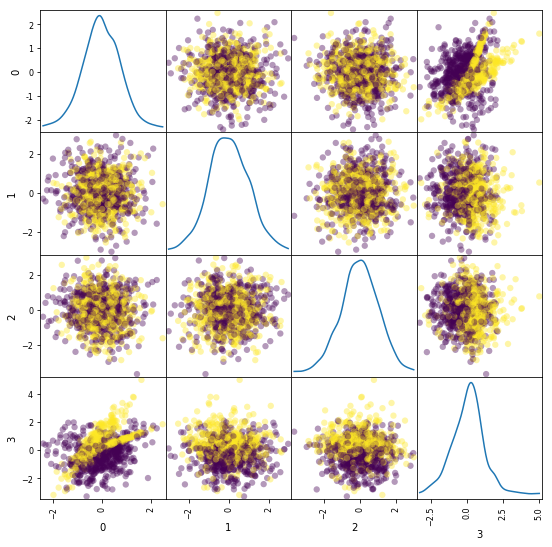
Synthesize a dataset of 10,000 4-vectors for binary classification with 2 informative features and 2 noise features.

X, y = sklearn.datasets.make_classification(
    n_samples=10000, n_features=4, n_redundant=0, n_informative=2, 
    n_clusters_per_class=2, hypercube=False, random_state=0
)
print 'data,',X.shape,y.shape # (10000, 4) (10000,) x0,x1,x2,x3, y

# Split into train and test
X, Xt, y, yt = sklearn.model_selection.train_test_split(X, y)
print 'train,',X.shape,y.shape  #train: (7500, 4) (7500,)
print 'test,', Xt.shape,yt.shape#test:  (2500, 4) (2500,)

# Visualize sample of the data
ind = np.random.permutation(X.shape[0])[:1000] # (7500,)--->(1000,)   x0,x1,x2,x3, y
df = pd.DataFrame(X[ind])
_ = pd.plotting.scatter_matrix(df, figsize=(9, 9), diagonal='kde', marker='o', s=40, alpha=.4, c=y[ind])

data, (10000, 4) (10000,)
train, (7500, 4) (7500,)
test, (2500, 4) (2500,)

Learn and evaluate scikit-learn's logistic regression with stochastic gradient descent (SGD) training. Time and check the classifier's accuracy.

%%timeit
# Train and test the scikit-learn SGD logistic regression.
clf = sklearn.linear_model.SGDClassifier(
    loss='log', n_iter=1000, penalty='l2', alpha=5e-4, class_weight='balanced')

clf.fit(X, y)
yt_pred = clf.predict(Xt)
print('Accuracy: {:.3f}'.format(sklearn.metrics.accuracy_score(yt, yt_pred)))

Accuracy: 0.781
Accuracy: 0.781
Accuracy: 0.781
Accuracy: 0.781
1 loop, best of 3: 372 ms per loop

Save the dataset to HDF5 for loading in Caffe.

# Write out the data to HDF5 files in a temp directory.
# This file is assumed to be caffe_root/examples/hdf5_classification.ipynb
dirname = os.path.abspath('./examples/hdf5_classification/data')
if not os.path.exists(dirname):
    os.makedirs(dirname)

train_filename = os.path.join(dirname, 'train.h5')
test_filename = os.path.join(dirname, 'test.h5')

# HDF5DataLayer source should be a file containing a list of HDF5 filenames.
# To show this off, we'll list the same data file twice.
with h5py.File(train_filename, 'w') as f:
    f['data'] = X
    f['label'] = y.astype(np.float32)
with open(os.path.join(dirname, 'train.txt'), 'w') as f:
    f.write(train_filename + '
')
    f.write(train_filename + '
')
    
# HDF5 is pretty efficient, but can be further compressed.
comp_kwargs = {'compression': 'gzip', 'compression_opts': 1}
with h5py.File(test_filename, 'w') as f:
    f.create_dataset('data', data=Xt, **comp_kwargs)
    f.create_dataset('label', data=yt.astype(np.float32), **comp_kwargs)
with open(os.path.join(dirname, 'test.txt'), 'w') as f:
    f.write(test_filename + '
')

Let's define logistic regression in Caffe through Python net specification. This is a quick and natural way to define nets that sidesteps manually editing the protobuf model.

from caffe import layers as L
from caffe import params as P

def logreg(hdf5, batch_size):
    # logistic regression: data, matrix multiplication, and 2-class softmax loss
    n = caffe.NetSpec()
    n.data, n.label = L.HDF5Data(batch_size=batch_size, source=hdf5, ntop=2)
    n.ip1 = L.InnerProduct(n.data, num_output=2, weight_filler=dict(type='xavier'))
    n.accuracy = L.Accuracy(n.ip1, n.label)
    n.loss = L.SoftmaxWithLoss(n.ip1, n.label)
    return n.to_proto()

train_net_path = 'examples/hdf5_classification/logreg_auto_train.prototxt'
with open(train_net_path, 'w') as f:
    f.write(str(logreg('examples/hdf5_classification/data/train.txt', 10)))

test_net_path = 'examples/hdf5_classification/logreg_auto_test.prototxt'
with open(test_net_path, 'w') as f:
    f.write(str(logreg('examples/hdf5_classification/data/test.txt', 10)))

Now, we'll define our "solver" which trains the network by specifying the locations of the train and test nets we defined above, as well as setting values for various parameters used for learning, display, and "snapshotting".

from caffe.proto import caffe_pb2

def solver(train_net_path, test_net_path):
    s = caffe_pb2.SolverParameter()

    # Specify locations of the train and test networks.
    s.train_net = train_net_path
    s.test_net.append(test_net_path)

    s.test_interval = 1000  # Test after every 1000 training iterations.
    s.test_iter.append(250) # Test 250 "batches" each time we test.

    s.max_iter = 10000      # # of times to update the net (training iterations)

    # Set the initial learning rate for stochastic gradient descent (SGD).
    s.base_lr = 0.01        

    # Set `lr_policy` to define how the learning rate changes during training.
    # Here, we 'step' the learning rate by multiplying it by a factor `gamma`
    # every `stepsize` iterations.
    s.lr_policy = 'step'
    s.gamma = 0.1
    s.stepsize = 5000

    # Set other optimization parameters. Setting a non-zero `momentum` takes a
    # weighted average of the current gradient and previous gradients to make
    # learning more stable. L2 weight decay regularizes learning, to help prevent
    # the model from overfitting.
    s.momentum = 0.9
    s.weight_decay = 5e-4

    # Display the current training loss and accuracy every 1000 iterations.
    s.display = 1000

    # Snapshots are files used to store networks we've trained.  Here, we'll
    # snapshot every 10K iterations -- just once at the end of training.
    # For larger networks that take longer to train, you may want to set
    # snapshot < max_iter to save the network and training state to disk during
    # optimization, preventing disaster in case of machine crashes, etc.
    s.snapshot = 10000
    s.snapshot_prefix = 'examples/hdf5_classification/data/train'

    # We'll train on the CPU for fair benchmarking against scikit-learn.
    # Changing to GPU should result in much faster training!
    s.solver_mode = caffe_pb2.SolverParameter.CPU
    
    return s

solver_path = 'examples/hdf5_classification/logreg_solver.prototxt'
with open(solver_path, 'w') as f:
    f.write(str(solver(train_net_path, test_net_path)))

Time to learn and evaluate our Caffeinated logistic regression in Python.

%%timeit
caffe.set_mode_cpu()
solver = caffe.get_solver(solver_path)
solver.solve()

accuracy = 0
batch_size = solver.test_nets[0].blobs['data'].num
test_iters = int(len(Xt) / batch_size)
for i in range(test_iters):
    solver.test_nets[0].forward()
    accuracy += solver.test_nets[0].blobs['accuracy'].data
accuracy /= test_iters

print("Accuracy: {:.3f}".format(accuracy))

Accuracy: 0.770
Accuracy: 0.770
Accuracy: 0.770
Accuracy: 0.770
1 loop, best of 3: 195 ms per loop

Do the same through the command line interface for detailed output on the model and solving.

!./build/tools/caffe train -solver examples/hdf5_classification/logreg_solver.prototxt

I0224 00:32:03.232779   655 caffe.cpp:178] Use CPU.
I0224 00:32:03.391911   655 solver.cpp:48] Initializing solver from parameters: 
train_net: "examples/hdf5_classification/logreg_auto_train.prototxt"
test_net: "examples/hdf5_classification/logreg_auto_test.prototxt"
......
I0224 00:32:04.087514   655 solver.cpp:406]     Test net output #0: accuracy = 0.77
I0224 00:32:04.087532   655 solver.cpp:406]     Test net output #1: loss = 0.593815 (* 1 = 0.593815 loss)
I0224 00:32:04.087541   655 solver.cpp:323] Optimization Done.
I0224 00:32:04.087548   655 caffe.cpp:222] Optimization Done.

If you look at output or the logreg_auto_train.prototxt, you'll see that the model is simple logistic regression.
We can make it a little more advanced by introducing a non-linearity between weights that take the input and weights that give the output -- now we have a two-layer network.
That network is given in nonlinear_auto_train.prototxt, and that's the only change made in nonlinear_logreg_solver.prototxt which we will now use.

The final accuracy of the new network should be higher than logistic regression!

from caffe import layers as L
from caffe import params as P

def nonlinear_net(hdf5, batch_size):
    # one small nonlinearity, one leap for model kind
    n = caffe.NetSpec()
    n.data, n.label = L.HDF5Data(batch_size=batch_size, source=hdf5, ntop=2)
    # define a hidden layer of dimension 40
    n.ip1 = L.InnerProduct(n.data, num_output=40, weight_filler=dict(type='xavier'))
    # transform the output through the ReLU (rectified linear) non-linearity
    n.relu1 = L.ReLU(n.ip1, in_place=True)
    # score the (now non-linear) features
    n.ip2 = L.InnerProduct(n.ip1, num_output=2, weight_filler=dict(type='xavier'))
    # same accuracy and loss as before
    n.accuracy = L.Accuracy(n.ip2, n.label)
    n.loss = L.SoftmaxWithLoss(n.ip2, n.label)
    return n.to_proto()

train_net_path = 'examples/hdf5_classification/nonlinear_auto_train.prototxt'
with open(train_net_path, 'w') as f:
    f.write(str(nonlinear_net('examples/hdf5_classification/data/train.txt', 10)))

test_net_path = 'examples/hdf5_classification/nonlinear_auto_test.prototxt'
with open(test_net_path, 'w') as f:
    f.write(str(nonlinear_net('examples/hdf5_classification/data/test.txt', 10)))

solver_path = 'examples/hdf5_classification/nonlinear_logreg_solver.prototxt'
with open(solver_path, 'w') as f:
    f.write(str(solver(train_net_path, test_net_path)))

%%timeit
caffe.set_mode_cpu()
solver = caffe.get_solver(solver_path)
solver.solve()

accuracy = 0
batch_size = solver.test_nets[0].blobs['data'].num
test_iters = int(len(Xt) / batch_size)
for i in range(test_iters):
    solver.test_nets[0].forward()
    accuracy += solver.test_nets[0].blobs['accuracy'].data
accuracy /= test_iters

print("Accuracy: {:.3f}".format(accuracy))

Accuracy: 0.838
Accuracy: 0.837
Accuracy: 0.838
Accuracy: 0.834
1 loop, best of 3: 277 ms per loop

Do the same through the command line interface for detailed output on the model and solving.

!./build/tools/caffe train -solver examples/hdf5_classification/nonlinear_logreg_solver.prototxt

I0224 00:32:05.654265   658 caffe.cpp:178] Use CPU.
I0224 00:32:05.810444   658 solver.cpp:48] Initializing solver from parameters: 
train_net: "examples/hdf5_classification/nonlinear_auto_train.prototxt"
test_net: "examples/hdf5_classification/nonlinear_auto_test.prototxt"
......
I0224 00:32:06.078208   658 solver.cpp:406]     Test net output #0: accuracy = 0.8388
I0224 00:32:06.078225   658 solver.cpp:406]     Test net output #1: loss = 0.382042 (* 1 = 0.382042 loss)
I0224 00:32:06.078234   658 solver.cpp:323] Optimization Done.
I0224 00:32:06.078241   658 caffe.cpp:222] Optimization Done.

# Clean up (comment this out if you want to examine the hdf5_classification/data directory).
shutil.rmtree(dirname)

Reference

• demo
• caffe git

History

• 20180102: created.

Copyright

• Post author: kezunlin
• Post link: https://kezunlin.me/post/c50b0018/
• Copyright Notice: All articles in this blog are licensed under CC BY-NC-SA 3.0 unless stating additionally.

Brewing Logistic Regression then Going Deeper.

Brewing Logistic Regression then Going Deeper

While Caffe is made for deep networks it can likewise represent "shallow" models like logistic regression for classification. We'll do simple logistic regression on synthetic data that we'll generate and save to HDF5 to feed vectors to Caffe. Once that model is done, we'll add layers to improve accuracy. That's what Caffe is about: define a model, experiment, and then deploy.

import numpy as np
import matplotlib.pyplot as plt
%matplotlib inline

import os
os.chdir('..')

import sys
sys.path.insert(0, './python')
import caffe


import os
import h5py
import shutil
import tempfile

import sklearn
import sklearn.datasets
import sklearn.linear_model

import pandas as pd

Synthesize a dataset of 10,000 4-vectors for binary classification with 2 informative features and 2 noise features.

X, y = sklearn.datasets.make_classification(
    n_samples=10000, n_features=4, n_redundant=0, n_informative=2, 
    n_clusters_per_class=2, hypercube=False, random_state=0
)
print 'data,',X.shape,y.shape # (10000, 4) (10000,) x0,x1,x2,x3, y

# Split into train and test
X, Xt, y, yt = sklearn.model_selection.train_test_split(X, y)
print 'train,',X.shape,y.shape  #train: (7500, 4) (7500,)
print 'test,', Xt.shape,yt.shape#test:  (2500, 4) (2500,)

# Visualize sample of the data
ind = np.random.permutation(X.shape[0])[:1000] # (7500,)--->(1000,)   x0,x1,x2,x3, y
df = pd.DataFrame(X[ind])
_ = pd.plotting.scatter_matrix(df, figsize=(9, 9), diagonal='kde', marker='o', s=40, alpha=.4, c=y[ind])

data, (10000, 4) (10000,)
train, (7500, 4) (7500,)
test, (2500, 4) (2500,)

Learn and evaluate scikit-learn's logistic regression with stochastic gradient descent (SGD) training. Time and check the classifier's accuracy.

%%timeit
# Train and test the scikit-learn SGD logistic regression.
clf = sklearn.linear_model.SGDClassifier(
    loss='log', n_iter=1000, penalty='l2', alpha=5e-4, class_weight='balanced')

clf.fit(X, y)
yt_pred = clf.predict(Xt)
print('Accuracy: {:.3f}'.format(sklearn.metrics.accuracy_score(yt, yt_pred)))

Accuracy: 0.781
Accuracy: 0.781
Accuracy: 0.781
Accuracy: 0.781
1 loop, best of 3: 372 ms per loop

Save the dataset to HDF5 for loading in Caffe.

# Write out the data to HDF5 files in a temp directory.
# This file is assumed to be caffe_root/examples/hdf5_classification.ipynb
dirname = os.path.abspath('./examples/hdf5_classification/data')
if not os.path.exists(dirname):
    os.makedirs(dirname)

train_filename = os.path.join(dirname, 'train.h5')
test_filename = os.path.join(dirname, 'test.h5')

# HDF5DataLayer source should be a file containing a list of HDF5 filenames.
# To show this off, we'll list the same data file twice.
with h5py.File(train_filename, 'w') as f:
    f['data'] = X
    f['label'] = y.astype(np.float32)
with open(os.path.join(dirname, 'train.txt'), 'w') as f:
    f.write(train_filename + '
')
    f.write(train_filename + '
')
    
# HDF5 is pretty efficient, but can be further compressed.
comp_kwargs = {'compression': 'gzip', 'compression_opts': 1}
with h5py.File(test_filename, 'w') as f:
    f.create_dataset('data', data=Xt, **comp_kwargs)
    f.create_dataset('label', data=yt.astype(np.float32), **comp_kwargs)
with open(os.path.join(dirname, 'test.txt'), 'w') as f:
    f.write(test_filename + '
')

Let's define logistic regression in Caffe through Python net specification. This is a quick and natural way to define nets that sidesteps manually editing the protobuf model.

from caffe import layers as L
from caffe import params as P

def logreg(hdf5, batch_size):
    # logistic regression: data, matrix multiplication, and 2-class softmax loss
    n = caffe.NetSpec()
    n.data, n.label = L.HDF5Data(batch_size=batch_size, source=hdf5, ntop=2)
    n.ip1 = L.InnerProduct(n.data, num_output=2, weight_filler=dict(type='xavier'))
    n.accuracy = L.Accuracy(n.ip1, n.label)
    n.loss = L.SoftmaxWithLoss(n.ip1, n.label)
    return n.to_proto()

train_net_path = 'examples/hdf5_classification/logreg_auto_train.prototxt'
with open(train_net_path, 'w') as f:
    f.write(str(logreg('examples/hdf5_classification/data/train.txt', 10)))

test_net_path = 'examples/hdf5_classification/logreg_auto_test.prototxt'
with open(test_net_path, 'w') as f:
    f.write(str(logreg('examples/hdf5_classification/data/test.txt', 10)))

Now, we'll define our "solver" which trains the network by specifying the locations of the train and test nets we defined above, as well as setting values for various parameters used for learning, display, and "snapshotting".

from caffe.proto import caffe_pb2

def solver(train_net_path, test_net_path):
    s = caffe_pb2.SolverParameter()

    # Specify locations of the train and test networks.
    s.train_net = train_net_path
    s.test_net.append(test_net_path)

    s.test_interval = 1000  # Test after every 1000 training iterations.
    s.test_iter.append(250) # Test 250 "batches" each time we test.

    s.max_iter = 10000      # # of times to update the net (training iterations)

    # Set the initial learning rate for stochastic gradient descent (SGD).
    s.base_lr = 0.01        

    # Set `lr_policy` to define how the learning rate changes during training.
    # Here, we 'step' the learning rate by multiplying it by a factor `gamma`
    # every `stepsize` iterations.
    s.lr_policy = 'step'
    s.gamma = 0.1
    s.stepsize = 5000

    # Set other optimization parameters. Setting a non-zero `momentum` takes a
    # weighted average of the current gradient and previous gradients to make
    # learning more stable. L2 weight decay regularizes learning, to help prevent
    # the model from overfitting.
    s.momentum = 0.9
    s.weight_decay = 5e-4

    # Display the current training loss and accuracy every 1000 iterations.
    s.display = 1000

    # Snapshots are files used to store networks we've trained.  Here, we'll
    # snapshot every 10K iterations -- just once at the end of training.
    # For larger networks that take longer to train, you may want to set
    # snapshot < max_iter to save the network and training state to disk during
    # optimization, preventing disaster in case of machine crashes, etc.
    s.snapshot = 10000
    s.snapshot_prefix = 'examples/hdf5_classification/data/train'

    # We'll train on the CPU for fair benchmarking against scikit-learn.
    # Changing to GPU should result in much faster training!
    s.solver_mode = caffe_pb2.SolverParameter.CPU
    
    return s

solver_path = 'examples/hdf5_classification/logreg_solver.prototxt'
with open(solver_path, 'w') as f:
    f.write(str(solver(train_net_path, test_net_path)))

Time to learn and evaluate our Caffeinated logistic regression in Python.

%%timeit
caffe.set_mode_cpu()
solver = caffe.get_solver(solver_path)
solver.solve()

accuracy = 0
batch_size = solver.test_nets[0].blobs['data'].num
test_iters = int(len(Xt) / batch_size)
for i in range(test_iters):
    solver.test_nets[0].forward()
    accuracy += solver.test_nets[0].blobs['accuracy'].data
accuracy /= test_iters

print("Accuracy: {:.3f}".format(accuracy))

Accuracy: 0.770
Accuracy: 0.770
Accuracy: 0.770
Accuracy: 0.770
1 loop, best of 3: 195 ms per loop

Do the same through the command line interface for detailed output on the model and solving.

!./build/tools/caffe train -solver examples/hdf5_classification/logreg_solver.prototxt

I0224 00:32:03.232779   655 caffe.cpp:178] Use CPU.
I0224 00:32:03.391911   655 solver.cpp:48] Initializing solver from parameters: 
train_net: "examples/hdf5_classification/logreg_auto_train.prototxt"
test_net: "examples/hdf5_classification/logreg_auto_test.prototxt"
......
I0224 00:32:04.087514   655 solver.cpp:406]     Test net output #0: accuracy = 0.77
I0224 00:32:04.087532   655 solver.cpp:406]     Test net output #1: loss = 0.593815 (* 1 = 0.593815 loss)
I0224 00:32:04.087541   655 solver.cpp:323] Optimization Done.
I0224 00:32:04.087548   655 caffe.cpp:222] Optimization Done.

If you look at output or the logreg_auto_train.prototxt, you'll see that the model is simple logistic regression.
We can make it a little more advanced by introducing a non-linearity between weights that take the input and weights that give the output -- now we have a two-layer network.
That network is given in nonlinear_auto_train.prototxt, and that's the only change made in nonlinear_logreg_solver.prototxt which we will now use.

The final accuracy of the new network should be higher than logistic regression!

from caffe import layers as L
from caffe import params as P

def nonlinear_net(hdf5, batch_size):
    # one small nonlinearity, one leap for model kind
    n = caffe.NetSpec()
    n.data, n.label = L.HDF5Data(batch_size=batch_size, source=hdf5, ntop=2)
    # define a hidden layer of dimension 40
    n.ip1 = L.InnerProduct(n.data, num_output=40, weight_filler=dict(type='xavier'))
    # transform the output through the ReLU (rectified linear) non-linearity
    n.relu1 = L.ReLU(n.ip1, in_place=True)
    # score the (now non-linear) features
    n.ip2 = L.InnerProduct(n.ip1, num_output=2, weight_filler=dict(type='xavier'))
    # same accuracy and loss as before
    n.accuracy = L.Accuracy(n.ip2, n.label)
    n.loss = L.SoftmaxWithLoss(n.ip2, n.label)
    return n.to_proto()

train_net_path = 'examples/hdf5_classification/nonlinear_auto_train.prototxt'
with open(train_net_path, 'w') as f:
    f.write(str(nonlinear_net('examples/hdf5_classification/data/train.txt', 10)))

test_net_path = 'examples/hdf5_classification/nonlinear_auto_test.prototxt'
with open(test_net_path, 'w') as f:
    f.write(str(nonlinear_net('examples/hdf5_classification/data/test.txt', 10)))

solver_path = 'examples/hdf5_classification/nonlinear_logreg_solver.prototxt'
with open(solver_path, 'w') as f:
    f.write(str(solver(train_net_path, test_net_path)))

%%timeit
caffe.set_mode_cpu()
solver = caffe.get_solver(solver_path)
solver.solve()

accuracy = 0
batch_size = solver.test_nets[0].blobs['data'].num
test_iters = int(len(Xt) / batch_size)
for i in range(test_iters):
    solver.test_nets[0].forward()
    accuracy += solver.test_nets[0].blobs['accuracy'].data
accuracy /= test_iters

print("Accuracy: {:.3f}".format(accuracy))

Accuracy: 0.838
Accuracy: 0.837
Accuracy: 0.838
Accuracy: 0.834
1 loop, best of 3: 277 ms per loop

Do the same through the command line interface for detailed output on the model and solving.

!./build/tools/caffe train -solver examples/hdf5_classification/nonlinear_logreg_solver.prototxt

I0224 00:32:05.654265   658 caffe.cpp:178] Use CPU.
I0224 00:32:05.810444   658 solver.cpp:48] Initializing solver from parameters: 
train_net: "examples/hdf5_classification/nonlinear_auto_train.prototxt"
test_net: "examples/hdf5_classification/nonlinear_auto_test.prototxt"
......
I0224 00:32:06.078208   658 solver.cpp:406]     Test net output #0: accuracy = 0.8388
I0224 00:32:06.078225   658 solver.cpp:406]     Test net output #1: loss = 0.382042 (* 1 = 0.382042 loss)
I0224 00:32:06.078234   658 solver.cpp:323] Optimization Done.
I0224 00:32:06.078241   658 caffe.cpp:222] Optimization Done.

# Clean up (comment this out if you want to examine the hdf5_classification/data directory).
shutil.rmtree(dirname)

Reference

• demo
• caffe git

History

• 20180102: created.

Copyright

• Post author: kezunlin
• Post link: https://kezunlin.me/post/c50b0018/
• Copyright Notice: All articles in this blog are licensed under CC BY-NC-SA 3.0 unless stating additionally.