《DSP using MATLAB》Problem 8.4

        今天是六一儿童节，陪伴不了家人，心里思念着他们，看着地里金黄的麦子，远处的山，高高的天

代码：

%% ------------------------------------------------------------------------
%%            Output Info about this m-file
fprintf('
***********************************************************
');
fprintf('        <DSP using MATLAB> Problem 8.4 

');
banner();
%% ------------------------------------------------------------------------

% digital Notch filter
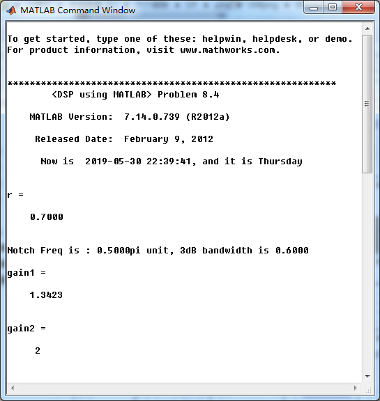
r = 0.7
%r = 0.9
%r = 0.99
omega0 = pi/2;

% corresponding system function  Direct form
b0 = 1.0;                                                                 % gain parameter
b   = b0*[1  -2*cos(omega0)  1];                                        % numerator with poles
a   = [1  -2*r*cos(omega0)   r*r];                                      % denominator 

% precise resonant frequency and 3dB bandwidth
omega_r = acos((1+r*r)*cos(omega0)/(2*r));
delta_omega = 2*(1-r);
fprintf('
Notch Freq is : %.4fpi unit, 3dB bandwidth is %.4f 
', omega_r/pi,delta_omega);
% 

[db, mag, pha, grd, w] = freqz_m(b, a);
[db_b, mag_b, pha_b, grd_b, w] = freqz_m(b, 1);

% ---------------------------------------------------------------------
%  Choose the gain parameter of the filter, maximum gain is equal to 1 
% ---------------------------------------------------------------------
gain1=max(mag)                    % with poles
gain2=max(mag_b)                  % without poles

[db, mag, pha, grd, w] = freqz_m(b/gain1, a);
[db_b, mag_b, pha_b, grd_b, w] = freqz_m(b/gain2, 1);

figure('NumberTitle', 'off', 'Name', 'Problem 8.4 Notch filter with poles')
set(gcf,'Color','white'); 

subplot(2,2,1); plot(w/pi, db); grid on; axis([0 2 -60 10]); 
set(gca,'YTickMode','manual','YTick',[-60,-30,0])
set(gca,'YTickLabelMode','manual','YTickLabel',['60';'30';' 0']);
set(gca,'XTickMode','manual','XTick',[0,0.5,1,1.5,2]);
xlabel('frequency in pi units'); ylabel('Decibels'); title('Magnitude Response in dB');

subplot(2,2,3); plot(w/pi, mag); grid on; %axis([0 1 -100 10]); 
xlabel('frequency in pi units'); ylabel('Absolute'); title('Magnitude Response in absolute');
set(gca,'XTickMode','manual','XTick',[0,0.5,1,1.5,2]);
set(gca,'YTickMode','manual','YTick',[0,1.0]);

subplot(2,2,2); plot(w/pi, pha); grid on; %axis([0 1 -100 10]); 
xlabel('frequency in pi units'); ylabel('Rad'); title('Phase Response in Radians');

subplot(2,2,4); plot(w/pi, grd*pi/180);  grid on; %axis([0 1 -100 10]); 
xlabel('frequency in pi units'); ylabel('Rad'); title('Group Delay');
set(gca,'XTickMode','manual','XTick',[0,0.5,1,1.5,2]);
%set(gca,'YTickMode','manual','YTick',[0,1.0]);


figure('NumberTitle', 'off', 'Name', 'Problem 8.4 Notch filter without poles')
set(gcf,'Color','white'); 

subplot(2,2,1); plot(w/pi, db_b); grid on; axis([0 2 -60 10]); 
set(gca,'YTickMode','manual','YTick',[-60,-30,0])
set(gca,'YTickLabelMode','manual','YTickLabel',['60';'30';' 0']);
set(gca,'XTickMode','manual','XTick',[0,0.25,0.5,1,1.5,1.75]);
xlabel('frequency in pi units'); ylabel('Decibels'); title('Magnitude Response in dB');

subplot(2,2,3); plot(w/pi, mag_b); grid on; %axis([0 1 -100 10]); 
xlabel('frequency in pi units'); ylabel('Absolute'); title('Magnitude Response in absolute');
set(gca,'XTickMode','manual','XTick',[0,0.5,1,1.5,2]);
set(gca,'YTickMode','manual','YTick',[0,1.0]);

subplot(2,2,2); plot(w/pi, pha_b); grid on; %axis([0 1 -100 10]); 
xlabel('frequency in pi units'); ylabel('Rad'); title('Phase Response in Radians');

subplot(2,2,4); plot(w/pi, grd_b*pi/180);  grid on; %axis([0 1 -100 10]); 
xlabel('frequency in pi units'); ylabel('Rad'); title('Group Delay');
set(gca,'XTickMode','manual','XTick',[0,0.5,1,1.5,2]);
%set(gca,'YTickMode','manual','YTick',[0,1.0]);


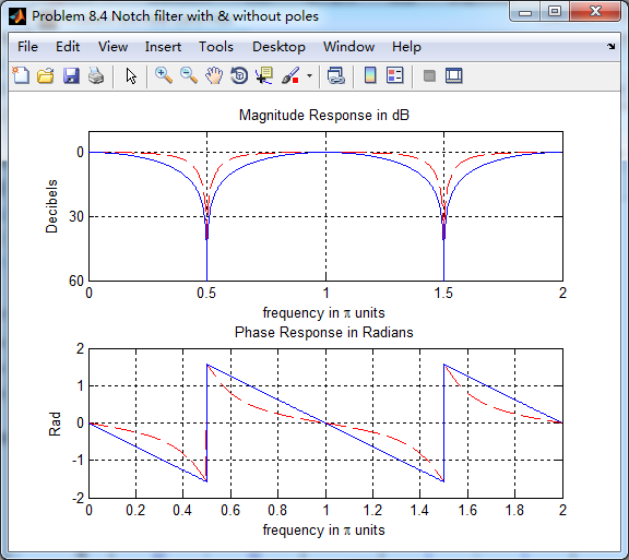
figure('NumberTitle', 'off', 'Name', 'Problem 8.4 Notch filter with & without poles')
set(gcf,'Color','white'); 

subplot(2,1,1); plot(w/pi, db, 'r--'); grid on; axis([0 2 -60 10]); hold on;
plot(w/pi, db_b); grid on; axis([0 2 -60 10]); hold off;
set(gca,'YTickMode','manual','YTick',[-60,-30,0])
set(gca,'YTickLabelMode','manual','YTickLabel',['60';'30';' 0']);
set(gca,'XTickMode','manual','XTick',[0,0.5,1,1.5,2]);
xlabel('frequency in pi units'); ylabel('Decibels'); title('Magnitude Response in dB');

subplot(2,1,2); plot(w/pi, pha, 'r--'); grid on; hold on;%axis([0 1 -100 10]); 
plot(w/pi, pha_b); hold off;
xlabel('frequency in pi units'); ylabel('Rad'); title('Phase Response in Radians');


figure('NumberTitle', 'off', 'Name', 'Problem 8.4 Pole-Zero Plot')
set(gcf,'Color','white'); 
zplane(b,a); 
title(sprintf('Pole-Zero Plot, r=%.2f  \omega=%.2f\pi',r,omega0/pi));
%pzplotz(b,a);

figure('NumberTitle', 'off', 'Name', 'Problem 8.4 Pole-Zero Plot')
set(gcf,'Color','white'); 
zplane(b,1); 
title(sprintf('Pole-Zero Plot, r=%.2f  \omega=%.2f\pi',r,omega0/pi));
%pzplotz(b,a);


% Impulse Response
fprintf('
----------------------------------');
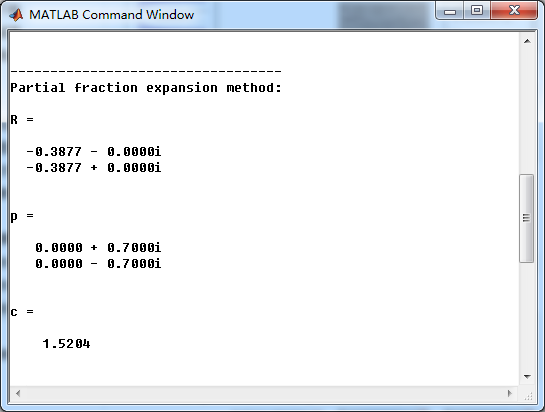
fprintf('
Partial fraction expansion method: 
');
b = b/gain1;
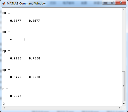
[R, p, c] = residuez(b , a)
MR = (abs(R))'              % Residue  Magnitude
AR = (angle(R))'/pi         % Residue  angles in pi units
Mp = (abs(p))'              % pole  Magnitude
Ap = (angle(p))'/pi         % pole  angles in pi units
[delta, n] = impseq(0,0,50);
h_chk = filter(b , a , delta);      % check sequences

% ------------------------------------------------------------------------
%              gain parameter b0=1
% ------------------------------------------------------------------------
h =  -0.5204*( 0.7.^n ) .* (2*cos(pi*n/2) ) + 2.0408 * delta;  % r=0.7
%h =   -0.1173*( 0.9.^n ) .* (2*cos(pi*n/2) ) + 1.2346 * delta;  % r=0.9
%h =  -0.0102*( 0.99.^n ) .* (2*cos(pi*n/2) ) + 1.0203 * delta;  % r=0.99
% ------------------------------------------------------------------------

% ------------------------------------------------------------------------
%              gain parameter b0 = equation
% ------------------------------------------------------------------------
%h =  -0.3877*( 0.7.^n ) .* (2*cos(pi*n/2) ) + 1.5204 * delta;  % r=0.7
%h =   -0.1173*( 0.9.^n ) .* (2*cos(pi*n/2) ) + 1.2346 * delta;  % r=0.9
%h =  -0.0102*( 0.99.^n ) .* (2*cos(pi*n/2) ) + 1.0203 * delta;  % r=0.99
% ------------------------------------------------------------------------

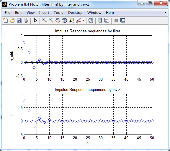
figure('NumberTitle', 'off', 'Name', 'Problem 8.4 Notch filter, h(n) by filter and Inv-Z ')
set(gcf,'Color','white'); 

subplot(2,1,1); stem(n, h_chk); grid on; %axis([0 2 -60 10]); 
xlabel('n'); ylabel('h\_chk'); title('Impulse Response sequences by filter');

subplot(2,1,2); stem(n, h/gain1); grid on; %axis([0 1 -100 10]); 
xlabel('n'); ylabel('h'); title('Impulse Response sequences by Inv-Z');


[db, mag, pha, grd, w] = freqz_m(h/gain1, [1]);


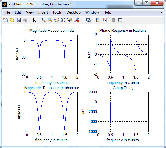
figure('NumberTitle', 'off', 'Name', 'Problem 8.4 Notch filter, h(n) by Inv-Z ')
set(gcf,'Color','white'); 

subplot(2,2,1); plot(w/pi, db); grid on; axis([0 2 -60 10]); 
set(gca,'YTickMode','manual','YTick',[-60,-30,0])
set(gca,'YTickLabelMode','manual','YTickLabel',['60';'30';' 0']);
set(gca,'XTickMode','manual','XTick',[0,0.5,1,1.5,2]);
xlabel('frequency in pi units'); ylabel('Decibels'); title('Magnitude Response in dB');

subplot(2,2,3); plot(w/pi, mag); grid on; %axis([0 1 -100 10]); 
xlabel('frequency in pi units'); ylabel('Absolute'); title('Magnitude Response in absolute');
set(gca,'XTickMode','manual','XTick',[0,0.5,1,1.5,2]);
set(gca,'YTickMode','manual','YTick',[0,1.0]);

subplot(2,2,2); plot(w/pi, pha); grid on; %axis([0 1 -100 10]); 
xlabel('frequency in pi units'); ylabel('Rad'); title('Phase Response in Radians');

subplot(2,2,4); plot(w/pi, grd*pi/180);  grid on; %axis([0 1 -100 10]); 
xlabel('frequency in pi units'); ylabel('Rad'); title('Group Delay');
set(gca,'XTickMode','manual','XTick',[0,0.5,1,1.5,2]);
%set(gca,'YTickMode','manual','YTick',[0,1.0]);


% Given resonat frequency and 3dB bandwidth
delta_omega = 0.04;
omega_r = pi*0.5;

r = 1 - delta_omega / 2

　　运行结果：

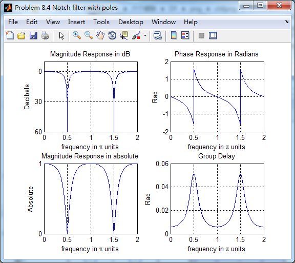
        陷波滤波器，ω0=0.5π，引入极点r=0.7

        系统函数部分分式展开

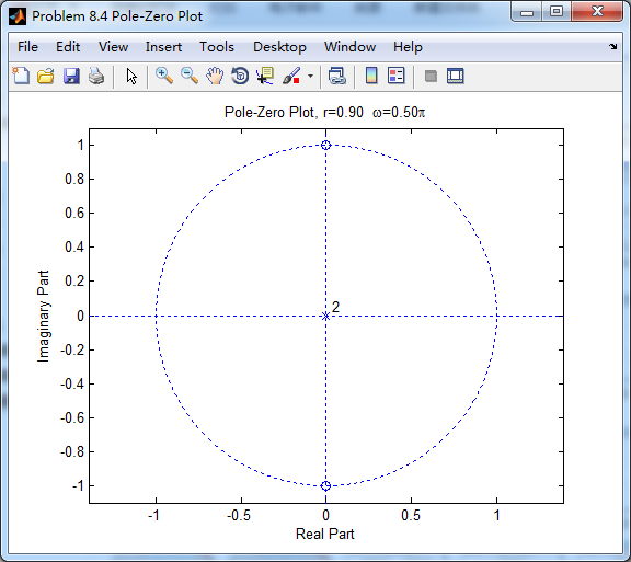
        系统零极点如下图

         幅度谱、相位谱、群延迟

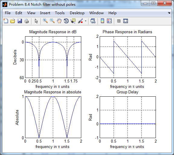
        零点位于原点位置，相当于去掉零点，如下

        去掉零点后，陷波滤波器的幅度谱、相位谱和群延迟

        引入零点的情况下，陷波频率附近频带更窄（红色），蓝色是无零点的情况。如同书上所言，陷波频率ω0

二者相差不大。

        系统函数部分分式展开后，查表，求逆z变换得到脉冲响应序列h(n)

        极点模r=0.9和0.99的结果，这里就不放了。