Linear Models
https://scikit-learn.org/stable/modules/linear_model.html#
线性模型,目标是特征的线性组合。有系数和偏置值。

Ordinary Least Squares
普通的最小均方差方法构造出来的模型, 就是 线性回归模型。

Linear Regression Example
https://scikit-learn.org/stable/auto_examples/linear_model/plot_ols.html#sphx-glr-auto-examples-linear-model-plot-ols-py
使用线性回归模型, 拟合糖尿病数据, 并绘制拟合曲线。
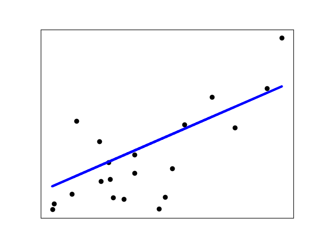
The example below uses only the first feature of the
diabetesdataset, in order to illustrate the data points within the two-dimensional plot. The straight line can be seen in the plot, showing how linear regression attempts to draw a straight line that will best minimize the residual sum of squares between the observed responses in the dataset, and the responses predicted by the linear approximation.The coefficients, residual sum of squares and the coefficient of determination are also calculated.
Out:
Coefficients:
 [938.23786125]
Mean squared error: 2548.07
Coefficient of determination: 0.47
print(__doc__)


# Code source: Jaques Grobler
# License: BSD 3 clause


import matplotlib.pyplot as plt
import numpy as np
from sklearn import datasets, linear_model
from sklearn.metrics import mean_squared_error, r2_score

# Load the diabetes dataset
diabetes_X, diabetes_y = datasets.load_diabetes(return_X_y=True)

# Use only one feature
diabetes_X = diabetes_X[:, np.newaxis, 2]

# Split the data into training/testing sets
diabetes_X_train = diabetes_X[:-20]
diabetes_X_test = diabetes_X[-20:]

# Split the targets into training/testing sets
diabetes_y_train = diabetes_y[:-20]
diabetes_y_test = diabetes_y[-20:]

# Create linear regression object
regr = linear_model.LinearRegression()

# Train the model using the training sets
regr.fit(diabetes_X_train, diabetes_y_train)

# Make predictions using the testing set
diabetes_y_pred = regr.predict(diabetes_X_test)

# The coefficients
print('Coefficients:
', regr.coef_)
# The mean squared error
print('Mean squared error: %.2f'
      % mean_squared_error(diabetes_y_test, diabetes_y_pred))
# The coefficient of determination: 1 is perfect prediction
print('Coefficient of determination: %.2f'
      % r2_score(diabetes_y_test, diabetes_y_pred))

# Plot outputs
plt.scatter(diabetes_X_test, diabetes_y_test,  color='black')
plt.plot(diabetes_X_test, diabetes_y_pred, color='blue', linewidth=3)

plt.xticks(())
plt.yticks(())

plt.show()
r2_score
https://scikit-learn.org/stable/modules/generated/sklearn.metrics.r2_score.html#sklearn.metrics.r2_score
此度量方法, 专门用于度量线性回归, 如果回归的结果方向完全相反, 则值为负数。
R^2 (coefficient of determination) regression score function.
Best possible score is 1.0 and it can be negative (because the model can be arbitrarily worse). A constant model that always predicts the expected value of y, disregarding the input features, would get a R^2 score of 0.0.
>>> from sklearn.metrics import r2_score
>>> y_true = [3, -0.5, 2, 7]
>>> y_pred = [2.5, 0.0, 2, 8]
>>> r2_score(y_true, y_pred)
0.948...
>>> y_true = [[0.5, 1], [-1, 1], [7, -6]]
>>> y_pred = [[0, 2], [-1, 2], [8, -5]]
>>> r2_score(y_true, y_pred,
...          multioutput='variance_weighted')
0.938...
>>> y_true = [1, 2, 3]
>>> y_pred = [1, 2, 3]
>>> r2_score(y_true, y_pred)
1.0
>>> y_true = [1, 2, 3]
>>> y_pred = [2, 2, 2]
>>> r2_score(y_true, y_pred)
0.0
>>> y_true = [1, 2, 3]
>>> y_pred = [3, 2, 1]
>>> r2_score(y_true, y_pred)
-3.0
Non-negative least squares
https://scikit-learn.org/stable/auto_examples/linear_model/plot_nnls.html#sphx-glr-auto-examples-linear-model-plot-nnls-py
对于线性回归模型,添加postive参数,可以保证系数不为负数。
Out:
Text(55.847222222222214, 0.5, 'NNLS regression coefficients')
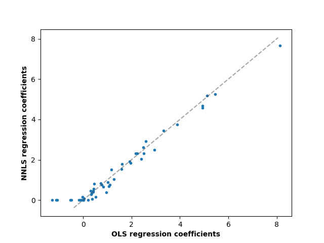
"""
==========================
Non-negative least squares
==========================

In this example, we fit a linear model with positive constraints on the
regression coefficients and compare the estimated coefficients to a classic
linear regression.
"""
print(__doc__)
import numpy as np
import matplotlib.pyplot as plt
from sklearn.metrics import r2_score

# %%
# Generate some random data
np.random.seed(42)

n_samples, n_features = 200, 50
X = np.random.randn(n_samples, n_features)
true_coef = 3 * np.random.randn(n_features)
# Threshold coefficients to render them non-negative
true_coef[true_coef < 0] = 0
y = np.dot(X, true_coef)

# Add some noise
y += 5 * np.random.normal(size=(n_samples, ))

# %%
# Split the data in train set and test set
from sklearn.model_selection import train_test_split

X_train, X_test, y_train, y_test = train_test_split(X, y, test_size=0.5)

# %%
# Fit the Non-Negative least squares.
from sklearn.linear_model import LinearRegression

reg_nnls = LinearRegression(positive=True)
y_pred_nnls = reg_nnls.fit(X_train, y_train).predict(X_test)
r2_score_nnls = r2_score(y_test, y_pred_nnls)
print("NNLS R2 score", r2_score_nnls)

# %%
# Fit an OLS.
reg_ols = LinearRegression()
y_pred_ols = reg_ols.fit(X_train, y_train).predict(X_test)
r2_score_ols = r2_score(y_test, y_pred_ols)
print("OLS R2 score", r2_score_ols)


# %%
# Comparing the regression coefficients between OLS and NNLS, we can observe
# they are highly correlated (the dashed line is the identity relation),
# but the non-negative constraint shrinks some to 0.
# The Non-Negative Least squares inherently yield sparse results.

fig, ax = plt.subplots()
ax.plot(reg_ols.coef_, reg_nnls.coef_, linewidth=0, marker=".")

low_x, high_x = ax.get_xlim()
low_y, high_y = ax.get_ylim()
low = max(low_x, low_y)
high = min(high_x, high_y)
ax.plot([low, high], [low, high], ls="--", c=".3", alpha=.5)
ax.set_xlabel("OLS regression coefficients", fontweight="bold")
ax.set_ylabel("NNLS regression coefficients", fontweight="bold")
Ridge regression and classification
岭回归是对线性回归的改进, 对于outlier,线性回归会非常敏感,导致部分系数可能超级大, 通过添加惩罚项目, 权重的L2范数, 来改善。
其变形可以用于分类问题。

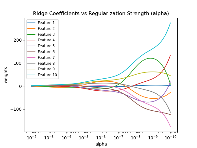
Plot Ridge coefficients as a function of the regularization
https://scikit-learn.org/stable/auto_examples/linear_model/plot_ridge_path.html#sphx-glr-auto-examples-linear-model-plot-ridge-path-py
岭回归,对于惩罚的力度,提供了调节参数。
如果下图效果, 如果惩罚力度越大, 靠左边部分, 回归系数都被惩罚为0.
Shows the effect of collinearity in the coefficients of an estimator.
RidgeRegression is the estimator used in this example. Each color represents a different feature of the coefficient vector, and this is displayed as a function of the regularization parameter.This example also shows the usefulness of applying Ridge regression to highly ill-conditioned matrices. For such matrices, a slight change in the target variable can cause huge variances in the calculated weights. In such cases, it is useful to set a certain regularization (alpha) to reduce this variation (noise).
When alpha is very large, the regularization effect dominates the squared loss function and the coefficients tend to zero. At the end of the path, as alpha tends toward zero and the solution tends towards the ordinary least squares, coefficients exhibit big oscillations. In practise it is necessary to tune alpha in such a way that a balance is maintained between both.
# Author: Fabian Pedregosa -- <fabian.pedregosa@inria.fr>
# License: BSD 3 clause

print(__doc__)

import numpy as np
import matplotlib.pyplot as plt
from sklearn import linear_model

# X is the 10x10 Hilbert matrix
X = 1. / (np.arange(1, 11) + np.arange(0, 10)[:, np.newaxis])
y = np.ones(10)

# #############################################################################
# Compute paths

n_alphas = 200
alphas = np.logspace(-10, -2, n_alphas)

coefs = []
for a in alphas:
    ridge = linear_model.Ridge(alpha=a, fit_intercept=False)
    ridge.fit(X, y)
    coefs.append(ridge.coef_)

# #############################################################################
# Display results

ax = plt.gca()

ax.plot(alphas, coefs)
ax.set_xscale('log')
ax.set_xlim(ax.get_xlim()[::-1])  # reverse axis
plt.xlabel('alpha')
plt.ylabel('weights')
plt.title('Ridge coefficients as a function of the regularization')
plt.axis('tight')
plt.show()
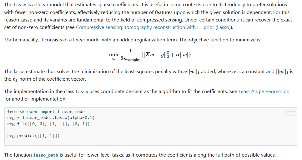
Lasso
此回归也是对线性回归的改进, 只不过于岭回归不同, 惩罚项是L1范式。
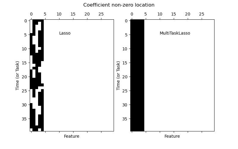
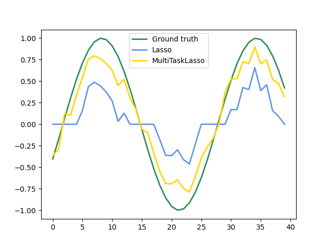
Joint feature selection with multi-task Lasso
https://scikit-learn.org/stable/auto_examples/linear_model/plot_multi_task_lasso_support.html#sphx-glr-auto-examples-linear-model-plot-multi-task-lasso-support-py
也存在多任务lasso回归,用于处理多目标回归问题。
The multi-task lasso allows to fit multiple regression problems jointly enforcing the selected features to be the same across tasks. This example simulates sequential measurements, each task is a time instant, and the relevant features vary in amplitude over time while being the same. The multi-task lasso imposes that features that are selected at one time point are select for all time point. This makes feature selection by the Lasso more stable.
print(__doc__)

# Author: Alexandre Gramfort <alexandre.gramfort@inria.fr>
# License: BSD 3 clause

import matplotlib.pyplot as plt
import numpy as np

from sklearn.linear_model import MultiTaskLasso, Lasso

rng = np.random.RandomState(42)

# Generate some 2D coefficients with sine waves with random frequency and phase
n_samples, n_features, n_tasks = 100, 30, 40
n_relevant_features = 5
coef = np.zeros((n_tasks, n_features))
times = np.linspace(0, 2 * np.pi, n_tasks)
for k in range(n_relevant_features):
    coef[:, k] = np.sin((1. + rng.randn(1)) * times + 3 * rng.randn(1))

X = rng.randn(n_samples, n_features)
Y = np.dot(X, coef.T) + rng.randn(n_samples, n_tasks)

coef_lasso_ = np.array([Lasso(alpha=0.5).fit(X, y).coef_ for y in Y.T])
coef_multi_task_lasso_ = MultiTaskLasso(alpha=1.).fit(X, Y).coef_

# #############################################################################
# Plot support and time series
fig = plt.figure(figsize=(8, 5))
plt.subplot(1, 2, 1)
plt.spy(coef_lasso_)
plt.xlabel('Feature')
plt.ylabel('Time (or Task)')
plt.text(10, 5, 'Lasso')
plt.subplot(1, 2, 2)
plt.spy(coef_multi_task_lasso_)
plt.xlabel('Feature')
plt.ylabel('Time (or Task)')
plt.text(10, 5, 'MultiTaskLasso')
fig.suptitle('Coefficient non-zero location')

feature_to_plot = 0
plt.figure()
lw = 2
plt.plot(coef[:, feature_to_plot], color='seagreen', linewidth=lw,
         label='Ground truth')
plt.plot(coef_lasso_[:, feature_to_plot], color='cornflowerblue', linewidth=lw,
         label='Lasso')
plt.plot(coef_multi_task_lasso_[:, feature_to_plot], color='gold', linewidth=lw,
         label='MultiTaskLasso')
plt.legend(loc='upper center')
plt.axis('tight')
plt.ylim([-1.1, 1.1])
plt.show()
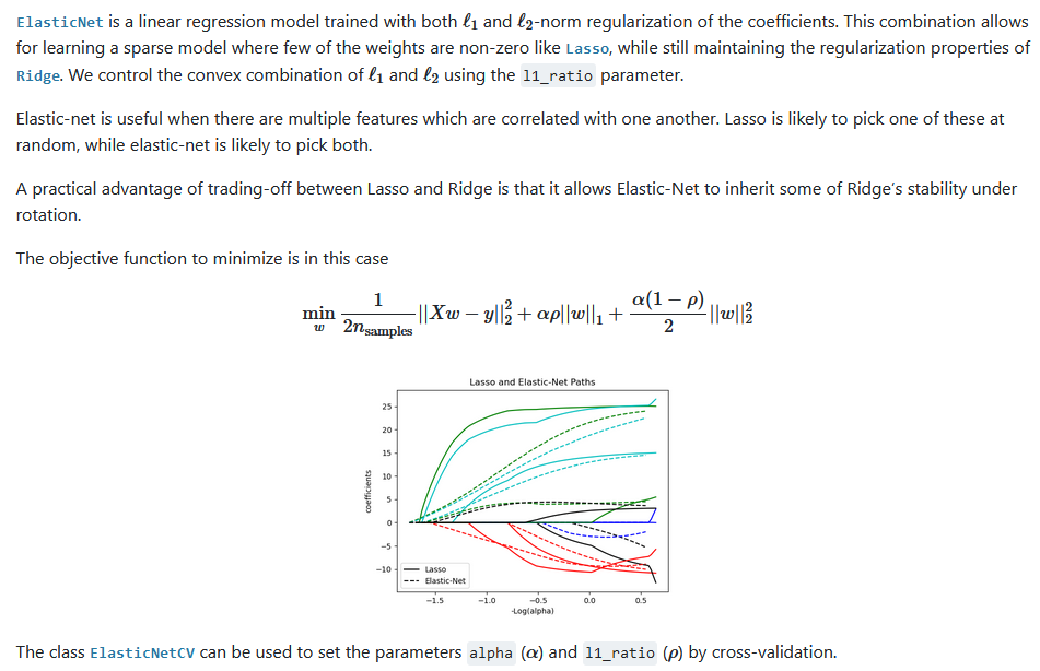
Elastic-Net
此回归是 岭回归 和 lasso回归的这种, 同时具有这两种惩罚项。
对于特征之间可能相关的情况, 此回归非常有用。
继承的岭回归的稳定性,也同时可以学习稀疏特征。
Bayesian Regression
Bayesian Ridge Regression
Bayesian Ridge Regression is used for regression:
>>> from sklearn import linear_model
>>> X = [[0., 0.], [1., 1.], [2., 2.], [3., 3.]]
>>> Y = [0., 1., 2., 3.]
>>> reg = linear_model.BayesianRidge()
>>> reg.fit(X, Y)
BayesianRidge()
After being fitted, the model can then be used to predict new values:
>>> reg.predict([[1, 0.]])
array([0.50000013])
The coefficients
of the model can be accessed:
>>> reg.coef_
array([0.49999993, 0.49999993])
Due to the Bayesian framework, the weights found are slightly different to the ones found by Ordinary Least Squares. However, Bayesian Ridge Regression is more robust to ill-posed problems.

Bayesian Ridge Regression
https://scikit-learn.org/stable/auto_examples/linear_model/plot_bayesian_ridge.html#sphx-glr-auto-examples-linear-model-plot-bayesian-ridge-py
于OLS方法, 贝叶斯岭回归方法,更加稳定。
Computes a Bayesian Ridge Regression on a synthetic dataset.
See Bayesian Ridge Regression for more information on the regressor.
Compared to the OLS (ordinary least squares) estimator, the coefficient weights are slightly shifted toward zeros, which stabilises them.
As the prior on the weights is a Gaussian prior, the histogram of the estimated weights is Gaussian.
The estimation of the model is done by iteratively maximizing the marginal log-likelihood of the observations.
We also plot predictions and uncertainties for Bayesian Ridge Regression for one dimensional regression using polynomial feature expansion. Note the uncertainty starts going up on the right side of the plot. This is because these test samples are outside of the range of the training samples.


print(__doc__)

import numpy as np
import matplotlib.pyplot as plt
from scipy import stats

from sklearn.linear_model import BayesianRidge, LinearRegression

# #############################################################################
# Generating simulated data with Gaussian weights
np.random.seed(0)
n_samples, n_features = 100, 100
X = np.random.randn(n_samples, n_features)  # Create Gaussian data
# Create weights with a precision lambda_ of 4.
lambda_ = 4.
w = np.zeros(n_features)
# Only keep 10 weights of interest
relevant_features = np.random.randint(0, n_features, 10)
for i in relevant_features:
    w[i] = stats.norm.rvs(loc=0, scale=1. / np.sqrt(lambda_))
# Create noise with a precision alpha of 50.
alpha_ = 50.
noise = stats.norm.rvs(loc=0, scale=1. / np.sqrt(alpha_), size=n_samples)
# Create the target
y = np.dot(X, w) + noise

# #############################################################################
# Fit the Bayesian Ridge Regression and an OLS for comparison
clf = BayesianRidge(compute_score=True)
clf.fit(X, y)

ols = LinearRegression()
ols.fit(X, y)

# #############################################################################
# Plot true weights, estimated weights, histogram of the weights, and
# predictions with standard deviations
lw = 2
plt.figure(figsize=(6, 5))
plt.title("Weights of the model")
plt.plot(clf.coef_, color='lightgreen', linewidth=lw,
         label="Bayesian Ridge estimate")
plt.plot(w, color='gold', linewidth=lw, label="Ground truth")
plt.plot(ols.coef_, color='navy', linestyle='--', label="OLS estimate")
plt.xlabel("Features")
plt.ylabel("Values of the weights")
plt.legend(loc="best", prop=dict(size=12))

plt.figure(figsize=(6, 5))
plt.title("Histogram of the weights")
plt.hist(clf.coef_, bins=n_features, color='gold', log=True,
         edgecolor='black')
plt.scatter(clf.coef_[relevant_features], np.full(len(relevant_features), 5.),
            color='navy', label="Relevant features")
plt.ylabel("Features")
plt.xlabel("Values of the weights")
plt.legend(loc="upper left")

plt.figure(figsize=(6, 5))
plt.title("Marginal log-likelihood")
plt.plot(clf.scores_, color='navy', linewidth=lw)
plt.ylabel("Score")
plt.xlabel("Iterations")


# Plotting some predictions for polynomial regression
def f(x, noise_amount):
    y = np.sqrt(x) * np.sin(x)
    noise = np.random.normal(0, 1, len(x))
    return y + noise_amount * noise


degree = 10
X = np.linspace(0, 10, 100)
y = f(X, noise_amount=0.1)
clf_poly = BayesianRidge()
clf_poly.fit(np.vander(X, degree), y)

X_plot = np.linspace(0, 11, 25)
y_plot = f(X_plot, noise_amount=0)
y_mean, y_std = clf_poly.predict(np.vander(X_plot, degree), return_std=True)
plt.figure(figsize=(6, 5))
plt.errorbar(X_plot, y_mean, y_std, color='navy',
             label="Polynomial Bayesian Ridge Regression", linewidth=lw)
plt.plot(X_plot, y_plot, color='gold', linewidth=lw,
         label="Ground Truth")
plt.ylabel("Output y")
plt.xlabel("Feature X")
plt.legend(loc="lower left")
plt.show()
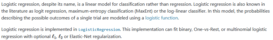
Logistic regression
逻辑回归是一个线性分类模型, 为啥叫逻辑回归呢, 因为其使用了 logit 回归函数, 最大熵分类或者是 log-linear分类器。
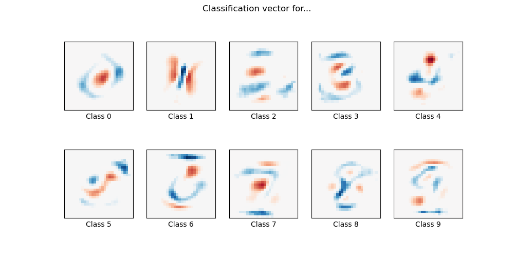
MNIST classification using multinomial logistic + L1
Here we fit a multinomial logistic regression with L1 penalty on a subset of the MNIST digits classification task. We use the SAGA algorithm for this purpose: this a solver that is fast when the number of samples is significantly larger than the number of features and is able to finely optimize non-smooth objective functions which is the case with the l1-penalty. Test accuracy reaches > 0.8, while weight vectors remains sparse and therefore more easily interpretable.
Note that this accuracy of this l1-penalized linear model is significantly below what can be reached by an l2-penalized linear model or a non-linear multi-layer perceptron model on this dataset.
Out:
Sparsity with L1 penalty: 79.95%
Test score with L1 penalty: 0.8322
Example run in 36.916 s
import time
import matplotlib.pyplot as plt
import numpy as np

from sklearn.datasets import fetch_openml
from sklearn.linear_model import LogisticRegression
from sklearn.model_selection import train_test_split
from sklearn.preprocessing import StandardScaler
from sklearn.utils import check_random_state

print(__doc__)

# Author: Arthur Mensch <arthur.mensch@m4x.org>
# License: BSD 3 clause

# Turn down for faster convergence
t0 = time.time()
train_samples = 5000

# Load data from https://www.openml.org/d/554
X, y = fetch_openml('mnist_784', version=1, return_X_y=True, as_frame=False)

random_state = check_random_state(0)
permutation = random_state.permutation(X.shape[0])
X = X[permutation]
y = y[permutation]
X = X.reshape((X.shape[0], -1))

X_train, X_test, y_train, y_test = train_test_split(
    X, y, train_size=train_samples, test_size=10000)

scaler = StandardScaler()
X_train = scaler.fit_transform(X_train)
X_test = scaler.transform(X_test)

# Turn up tolerance for faster convergence
clf = LogisticRegression(
    C=50. / train_samples, penalty='l1', solver='saga', tol=0.1
)
clf.fit(X_train, y_train)
sparsity = np.mean(clf.coef_ == 0) * 100
score = clf.score(X_test, y_test)
# print('Best C % .4f' % clf.C_)
print("Sparsity with L1 penalty: %.2f%%" % sparsity)
print("Test score with L1 penalty: %.4f" % score)

coef = clf.coef_.copy()
plt.figure(figsize=(10, 5))
scale = np.abs(coef).max()
for i in range(10):
    l1_plot = plt.subplot(2, 5, i + 1)
    l1_plot.imshow(coef[i].reshape(28, 28), interpolation='nearest',
                   cmap=plt.cm.RdBu, vmin=-scale, vmax=scale)
    l1_plot.set_xticks(())
    l1_plot.set_yticks(())
    l1_plot.set_xlabel('Class %i' % i)
plt.suptitle('Classification vector for...')

run_time = time.time() - t0
print('Example run in %.3f s' % run_time)
plt.show()