1.动机 - (Motivation)
卷积神经网络(CNN)是多层前向网络(MLPs)的一种变体,而MLP是受生物学的启发发展而来的。从Hubel和Wiesel对猫的视觉皮层(visual contex)所做的早期工作,我们可以看出视觉皮层中的神经元(cells)分布十分复杂。每个神经元仅对视觉域(visual field)的某个局部区域较为敏感,这个区域叫做感受野(receptive field)。这些局部区域以平铺方式覆盖整个视觉域。这些神经元对于输入空间(input space)表现为局部滤波器(local filter)的特性,并且适用于挖掘存在于自然图像中的局部空间关系信息。
更多地,有两种基本的神经元类型:简单神经元(Simple cell)在自身感受野内,可以对特定的边缘模式(edge-like patterns)产生最大化的相应。而复杂神经元(Complex cell)具有更大的感受野,并对模式的精确位置具有局部不变性(locally invariant)。
动物的视觉层皮是现有的最强大的视觉处理系统,因此效仿视觉皮层的行为是很自然的想法。所以,有许多受到神经元工作原理启发而发表的文章。例如:NeoCognitron[Fukushima],HMAX[Serre07] and LeNet-5 [LeCun98],本课程重点讨论LeNet-5。
2.稀疏连接性 - (Sparse Connectivity)
CNN是通过相邻层神经元之间的局部连接,挖掘空间上的局部关联性(local correlation)。换句话说,m层隐单元(hidden units)的输入,来源于m-1层部分单元的输出,而这些单元具有空间上连续的感受野。我们可以看下图说明:
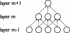
假如,m-1层是视网膜输入层。在上图中,m层的单元在视网膜层有宽度为3的感受野,所以m层的单元仅和视网膜层相邻的3个神经元连接。m+1层具有与m层相似的连接关系。我们可以说,m+1层关于m层的感受野为3,而m+1层关于输入层的感受野为5。每个单元对于其感受野以外的变化不作相应。因此这种架构可以确保,学习到的“滤波器”对于"空间局部输入模式"能产生最强的相应。
如上图可示,堆砌许多这样的“层”可以获得一个(非线性)"滤波器(filters)",且这种滤波器会变得更具“全局性(global)”(也就是说,可以对像素空间中很大范围都产生相应)。例如,m+1层的隐单元可以编码一个宽度为5的非线性特征(就像素空间而言)。
3.共享权值 - (Shared Weights)
在CNN中,每个滤波器 在整个视觉域(visual field)上是不断重复的。这些重复的单元共享着相同的参数设定(权值向量(weight
vector)和偏置(bias)),并且组成一个特征图(feature map)。
在整个视觉域(visual field)上是不断重复的。这些重复的单元共享着相同的参数设定(权值向量(weight
vector)和偏置(bias)),并且组成一个特征图(feature map)。
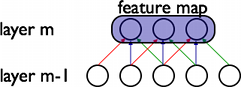
在上图中,展示了属于同一个特征图的3个隐节点。相同颜色的权值是共享的——被约束成恒等。梯度下降法(Gradient descent)仍然可以用来学习这些共享的参数,只需要对原始的算法进行略微的修改。共享权值的梯度简单地等于共享参数梯度之和。
以这种形式重复放置神经元,可以更好地检测特征,而无需在意特征在视觉域上的位置。此外,权值共享提高了学习的效率,因为权值共享大大减少了参数学习的个数。“共享权值”约束,使得CNN在解决视觉问题中具有更佳的通用特性。
4.细节及标注说明 - (Details and Notation)
对整个图像的局部区域重复应用一个函数,可以获得一个特征图。换句话说,也就是用线性滤波器对图像进行卷积,加上一个偏置,再应用一个非线性的函数。如果我们将给定层的第k个特征图记为 ,这个特征图由权值向量
 和偏置
和偏置 得到,再经过
 非线性函数。

|
Note
回忆一维信号卷积的定义式:![o[n] = f[n]*g[n] = sum_{u=-infty}^{infty} f[u] g[n-u] = sum_{u=-infty}^{infty} f[n-u] g[u]](http://deeplearning.net/tutorial/_images/math/ebecd534421ecfe888609e0d78943c8616e222e5.png) . .上式可以扩展到二维形式: ![o[m,n] = f[m,n]*g[m,n] = sum_{u=-infty}^{infty} sum_{v=-infty}^{infty} f[u,v] g[m-u,n-v]](http://deeplearning.net/tutorial/_images/math/018bdc7d2f74411a1895e3075ffb0c6cbe4c7521.png) . . |
为了以更加丰富的方式表征数据,每个隐层由多个特征图组成,记为 ,隐层的权值
 可以表示为一个四维张量(4D
tensor),这个张量内的元素反应了四个维度的每种组合:目标特征图(destination feature map),源特征图(source feature map),源垂直位置(source vertical position)和源水平位置(source horizontal position)。偏置
可以表示为一个四维张量(4D
tensor),这个张量内的元素反应了四个维度的每种组合:目标特征图(destination feature map),源特征图(source feature map),源垂直位置(source vertical position)和源水平位置(source horizontal position)。偏置 可以表示为一个一维向量,这个维度是指目标特征图。我们以下图说明:
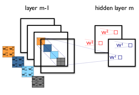
图一 一个卷积层的实例
图中画了一个CNN的两层示意图。m-1层包含4个特征图,m隐层含有2个特征图( 和
和 )。
和 中的像素(神经元输出,用蓝/红方块标出)是由m-1层的像素以2x2的感受野(用彩色方块标出)计算而来。注意感受野是如何跨越这四个输入特征图的。所以
和 的权重
)。
和 中的像素(神经元输出,用蓝/红方块标出)是由m-1层的像素以2x2的感受野(用彩色方块标出)计算而来。注意感受野是如何跨越这四个输入特征图的。所以
和 的权重 和
和 是三维张量。一个维度用于表示输入特征图,其他两个维度用于表示像素坐标。
汇总而言,连接 "m层第k个特征图像素" 和 "m-1层第l个特征图上坐标为(i,j)的像素" 的权重记为 。
。
5.卷积操作 - (The Convolution Operator)
ConvOp是实现卷积层的主要工具。ConvOp被theano.tensor.signal.conv2d使用,有两个输入参数:
- 一小批输入图像
所对应的四维张量。四维张量的形式:[一小批的数量,输入特征图数量,图像高度,图像宽度]。 - 权值矩阵 所对应的四维张量。四维张量的形式:[m层特征图数量,m-1层特征图数量,滤波器高度,滤波器宽度]。
以下是Theano用于实现卷积层(类似于图一)的代码。输入包含三个特征图(RGB彩色图),大小为120x160。我们使用两个9x9感受野的卷积滤波器。
import theano
from theano import tensor as T
from theano.tensor.nnet import conv

import numpy

rng = numpy.random.RandomState(23455)

# instantiate 4D tensor for input
input = T.tensor4(name='input')

# initialize shared variable for weights.
w_shp = (2, 3, 9, 9)
w_bound = numpy.sqrt(3 * 9 * 9)
W = theano.shared( numpy.asarray(
            rng.uniform(
                low=-1.0 / w_bound,
                high=1.0 / w_bound,
                size=w_shp),
            dtype=input.dtype), name ='W')

# initialize shared variable for bias (1D tensor) with random values
# IMPORTANT: biases are usually initialized to zero. However in this
# particular application, we simply apply the convolutional layer to
# an image without learning the parameters. We therefore initialize
# them to random values to "simulate" learning.
b_shp = (2,)
b = theano.shared(numpy.asarray(
            rng.uniform(low=-.5, high=.5, size=b_shp),
            dtype=input.dtype), name ='b')

# build symbolic expression that computes the convolution of input with filters in w
conv_out = conv.conv2d(input, W)

# build symbolic expression to add bias and apply activation function, i.e. produce neural net layer output
# A few words on ``dimshuffle`` :
#   ``dimshuffle`` is a powerful tool in reshaping a tensor;
#   what it allows you to do is to shuffle dimension around
#   but also to insert new ones along which the tensor will be
#   broadcastable;
#   dimshuffle('x', 2, 'x', 0, 1)
#   This will work on 3d tensors with no broadcastable
#   dimensions. The first dimension will be broadcastable,
#   then we will have the third dimension of the input tensor as
#   the second of the resulting tensor, etc. If the tensor has
#   shape (20, 30, 40), the resulting tensor will have dimensions
#   (1, 40, 1, 20, 30). (AxBxC tensor is mapped to 1xCx1xAxB tensor)
#   More examples:
#    dimshuffle('x') -> make a 0d (scalar) into a 1d vector
#    dimshuffle(0, 1) -> identity
#    dimshuffle(1, 0) -> inverts the first and second dimensions
#    dimshuffle('x', 0) -> make a row out of a 1d vector (N to 1xN)
#    dimshuffle(0, 'x') -> make a column out of a 1d vector (N to Nx1)
#    dimshuffle(2, 0, 1) -> AxBxC to CxAxB
#    dimshuffle(0, 'x', 1) -> AxB to Ax1xB
#    dimshuffle(1, 'x', 0) -> AxB to Bx1xA
output = T.nnet.sigmoid(conv_out + b.dimshuffle('x', 0, 'x', 'x'))

# create theano function to compute filtered images
f = theano.function([input], output)
让我们用以下代码完成点有趣的事情...
import numpy
import pylab
from PIL import Image

# open random image of dimensions 639x516
img = Image.open(open('doc/images/3wolfmoon.jpg'))
# dimensions are (height, width, channel)
img = numpy.asarray(img, dtype='float64') / 256.

# put image in 4D tensor of shape (1, 3, height, width)
img_ = img.transpose(2, 0, 1).reshape(1, 3, 639, 516)
filtered_img = f(img_)

# plot original image and first and second components of output
pylab.subplot(1, 3, 1); pylab.axis('off'); pylab.imshow(img)
pylab.gray();
# recall that the convOp output (filtered image) is actually a "minibatch",
# of size 1 here, so we take index 0 in the first dimension:
pylab.subplot(1, 3, 2); pylab.axis('off'); pylab.imshow(filtered_img[0, 0, :, :])
pylab.subplot(1, 3, 3); pylab.axis('off'); pylab.imshow(filtered_img[0, 1, :, :])
pylab.show()
这将产生以下的输出:
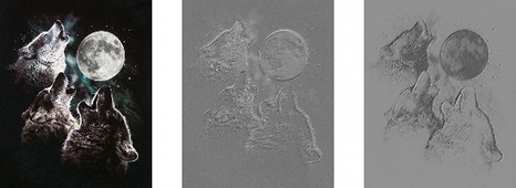
注意到,一个随机初始化的滤波器效果非常类似于边缘检测器(edge detector)!
我们使用了和MLP一样的权值初始化公式。权值在[-1/fan-in,1/fan-in]范围的均匀分布上随机采样,其中fan-in是隐单元的输入数。对于MLP,它是前层的单元数。对于CNNs,我们不得不考虑输入特征图数量和感受野的大小。
6.最大池化 - (Maxpooling)
CNN的另一个非常重要的概念叫做最大池化(Max-pooling),它是某种形式的非线性降采样(non-linear down-sampling)。最大池化将输入图像划分为一系列不重叠(non-overlapping)的矩形,对于每个矩形区域,输出是其区域的最大值。
最大池化对视觉处理非常有用,原因如下:
- 通过移除非最大值(non-maximal value),减少了后层运算量。
- 它提供了一种形式的平移不变性。想象一下将最大池化层(max-pooling layer)与卷积层(convolutional layer)级联。原本输入图像的单一像素点可以在8个方向上做平移变换。如果采用2x2的区域做最大池化,那么有3种平移变换的池化效果将与卷积层输出完全一致。如果采用5x5的区域做最大池化,那么准确的概率变为5/8。由于池化能提供对于位置变化的鲁棒性,因此,最大池化是一种减少中间级维数的“巧妙”方式。
Theano通过theano.tensor.signal.downsample.max_pool_2d的方式完成最大池化。这个函数的输入参数为:一个N维张量(其中N>=2),降采样因子(downscaling
factor)。并对张量的后两个维度做最大池化。
"An example is worth a thousand words."
from theano.tensor.signal import downsample

input = T.dtensor4('input')
maxpool_shape = (2, 2)
pool_out = downsample.max_pool_2d(input, maxpool_shape, ignore_border=True)
f = theano.function([input],pool_out)

invals = numpy.random.RandomState(1).rand(3, 2, 5, 5)
print 'With ignore_border set to True:'
print 'invals[0, 0, :, :] =
', invals[0, 0, :, :]
print 'output[0, 0, :, :] =
', f(invals)[0, 0, :, :]

pool_out = downsample.max_pool_2d(input, maxpool_shape, ignore_border=False)
f = theano.function([input],pool_out)
print 'With ignore_border set to False:'
print 'invals[1, 0, :, :] =
 ', invals[1, 0, :, :]
print 'output[1, 0, :, :] =
', f(invals)[1, 0, :, :]With ignore_border set to True:
invals[0, 0, :, :] =
[[ 4.17022005e-01 7.20324493e-01 1.14374817e-04 3.02332573e-01 1.46755891e-01]
[ 9.23385948e-02 1.86260211e-01 3.45560727e-01 3.96767474e-01 5.38816734e-01]
[ 4.19194514e-01 6.85219500e-01 2.04452250e-01 8.78117436e-01 2.73875932e-02]
[ 6.70467510e-01 4.17304802e-01 5.58689828e-01 1.40386939e-01 1.98101489e-01]
[ 8.00744569e-01 9.68261576e-01 3.13424178e-01 6.92322616e-01 8.76389152e-01]]
output[0, 0, :, :] =
[[ 0.72032449 0.39676747]
[ 0.6852195 0.87811744]]
With ignore_border set to False:
invals[1, 0, :, :] =
[[ 0.01936696 0.67883553 0.21162812 0.26554666 0.49157316]
[ 0.05336255 0.57411761 0.14672857 0.58930554 0.69975836]
[ 0.10233443 0.41405599 0.69440016 0.41417927 0.04995346]
[ 0.53589641 0.66379465 0.51488911 0.94459476 0.58655504]
[ 0.90340192 0.1374747 0.13927635 0.80739129 0.39767684]]
output[1, 0, :, :] =
[[ 0.67883553 0.58930554 0.69975836]
[ 0.66379465 0.94459476 0.58655504]
[ 0.90340192 0.80739129 0.39767684]]max_pool_2d操作有一点"特殊"。程序在图像生成时,必须知道降采样因子ds(一个二元组,分别记录了图像宽度和高度降采样因子)。这将在未来版本中改变。
7.一个完整模型:LeNet
稀疏,卷积层和最大池化,是LeNet这类模型的核心。而每个模型的实际细节大有不同,下图刻画了LeNet的图解。
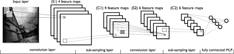
前面几层由交替的卷积层和最大池化层组成。然而,后面几层是全连接(fully-connected)层,相当于一个传统的MLP(隐层(hidden layer)+逻辑回归(logistic regression))。第一个全连接层的输入是前一层所有特征图的集合。
从应用的角度出发,这意味着前面几层是以四维张量进行操作。然后这些四维张量被整理成栅格状特征图的二维矩阵形式,这样可以兼容MLP的实现。
|
Note
需要注意,名词“卷积”可能对应于不同的数学操作:
|
8.融会贯通 - (Putting it All Together)
如今,我们已经有了实现LeNet模型所需的各个组件。我们还需要LeNetConvPoolLayer类,用于实现一个{卷积+最大池化}层。
class LeNetConvPoolLayer(object):
    """Pool Layer of a convolutional network """

    def __init__(self, rng, input, filter_shape, image_shape, poolsize=(2, 2)):
        """
        Allocate a LeNetConvPoolLayer with shared variable internal parameters.

        :type rng: numpy.random.RandomState
        :param rng: a random number generator used to initialize weights

        :type input: theano.tensor.dtensor4
        :param input: symbolic image tensor, of shape image_shape

        :type filter_shape: tuple or list of length 4
        :param filter_shape: (number of filters, num input feature maps,
                              filter height, filter width)

        :type image_shape: tuple or list of length 4
        :param image_shape: (batch size, num input feature maps,
                             image height, image width)

        :type poolsize: tuple or list of length 2
        :param poolsize: the downsampling (pooling) factor (#rows, #cols)
        """

        assert image_shape[1] == filter_shape[1]
        self.input = input

        # there are "num input feature maps * filter height * filter width"
        # inputs to each hidden unit
        fan_in = numpy.prod(filter_shape[1:])
        # each unit in the lower layer receives a gradient from:
        # "num output feature maps * filter height * filter width" /
        #   pooling size
        fan_out = (filter_shape[0] * numpy.prod(filter_shape[2:]) /
                   numpy.prod(poolsize))
        # initialize weights with random weights
        W_bound = numpy.sqrt(6. / (fan_in + fan_out))
        self.W = theano.shared(
            numpy.asarray(
                rng.uniform(low=-W_bound, high=W_bound, size=filter_shape),
                dtype=theano.config.floatX
            ),
            borrow=True
        )

        # the bias is a 1D tensor -- one bias per output feature map
        b_values = numpy.zeros((filter_shape[0],), dtype=theano.config.floatX)
        self.b = theano.shared(value=b_values, borrow=True)

        # convolve input feature maps with filters
        conv_out = conv.conv2d(
            input=input,
            filters=self.W,
            filter_shape=filter_shape,
            image_shape=image_shape
        )

        # downsample each feature map individually, using maxpooling
        pooled_out = downsample.max_pool_2d(
            input=conv_out,
            ds=poolsize,
            ignore_border=True
        )

        # add the bias term. Since the bias is a vector (1D array), we first
        # reshape it to a tensor of shape (1, n_filters, 1, 1). Each bias will
        # thus be broadcasted across mini-batches and feature map
        # width & height
        self.output = T.tanh(pooled_out + self.b.dimshuffle('x', 0, 'x', 'x'))

        # store parameters of this layer
        self.params = [self.W, self.b]

        # keep track of model input
self.input = inputfan-in值由感受野的大小,以及输入特征图的个数决定。
最终,使用Classifying
MNIST digits using Logistic Regression中定义的LogisticRegression类,以及中Multilayer
Perceptron定义的HiddenLayer类。我们实例化以下这个网络:
    x = T.matrix('x')   # the data is presented as rasterized images
    y = T.ivector('y')  # the labels are presented as 1D vector of
                        # [int] labels

    ######################
    # BUILD ACTUAL MODEL #
    ######################
    print '... building the model'

    # Reshape matrix of rasterized images of shape (batch_size, 28 * 28)
    # to a 4D tensor, compatible with our LeNetConvPoolLayer
    # (28, 28) is the size of MNIST images.
    layer0_input = x.reshape((batch_size, 1, 28, 28))

    # Construct the first convolutional pooling layer:
    # filtering reduces the image size to (28-5+1 , 28-5+1) = (24, 24)
    # maxpooling reduces this further to (24/2, 24/2) = (12, 12)
    # 4D output tensor is thus of shape (batch_size, nkerns[0], 12, 12)
    layer0 = LeNetConvPoolLayer(
        rng,
        input=layer0_input,
        image_shape=(batch_size, 1, 28, 28),
        filter_shape=(nkerns[0], 1, 5, 5),
        poolsize=(2, 2)
    )

    # Construct the second convolutional pooling layer
    # filtering reduces the image size to (12-5+1, 12-5+1) = (8, 8)
    # maxpooling reduces this further to (8/2, 8/2) = (4, 4)
    # 4D output tensor is thus of shape (batch_size, nkerns[1], 4, 4)
    layer1 = LeNetConvPoolLayer(
        rng,
        input=layer0.output,
        image_shape=(batch_size, nkerns[0], 12, 12),
        filter_shape=(nkerns[1], nkerns[0], 5, 5),
        poolsize=(2, 2)
    )

    # the HiddenLayer being fully-connected, it operates on 2D matrices of
    # shape (batch_size, num_pixels) (i.e matrix of rasterized images).
    # This will generate a matrix of shape (batch_size, nkerns[1] * 4 * 4),
    # or (500, 50 * 4 * 4) = (500, 800) with the default values.
    layer2_input = layer1.output.flatten(2)

    # construct a fully-connected sigmoidal layer
    layer2 = HiddenLayer(
        rng,
        input=layer2_input,
        n_in=nkerns[1] * 4 * 4,
        n_out=500,
        activation=T.tanh
    )

    # classify the values of the fully-connected sigmoidal layer
    layer3 = LogisticRegression(input=layer2.output, n_in=500, n_out=10)

    # the cost we minimize during training is the NLL of the model
    cost = layer3.negative_log_likelihood(y)

    # create a function to compute the mistakes that are made by the model
    test_model = theano.function(
        [index],
        layer3.errors(y),
        givens={
            x: test_set_x[index * batch_size: (index + 1) * batch_size],
            y: test_set_y[index * batch_size: (index + 1) * batch_size]
        }
    )

    validate_model = theano.function(
        [index],
        layer3.errors(y),
        givens={
            x: valid_set_x[index * batch_size: (index + 1) * batch_size],
            y: valid_set_y[index * batch_size: (index + 1) * batch_size]
        }
    )

    # create a list of all model parameters to be fit by gradient descent
    params = layer3.params + layer2.params + layer1.params + layer0.params

    # create a list of gradients for all model parameters
    grads = T.grad(cost, params)

    # train_model is a function that updates the model parameters by
    # SGD Since this model has many parameters, it would be tedious to
    # manually create an update rule for each model parameter. We thus
    # create the updates list by automatically looping over all
    # (params[i], grads[i]) pairs.
    updates = [
        (param_i, param_i - learning_rate * grad_i)
        for param_i, grad_i in zip(params, grads)
    ]

    train_model = theano.function(
        [index],
        cost,
        updates=updates,
        givens={
            x: train_set_x[index * batch_size: (index + 1) * batch_size],
            y: train_set_y[index * batch_size: (index + 1) * batch_size]
        }
    )
我们不考虑实际训练和终止条件的代码,因为它和MLP的代码完全一致。有兴趣的读者可以在DeepLearning教程的code文件夹获取代码。
9.运行代码 - (Running the Code)
用户可以通过以下命令调用代码:
python code/convolutional_mlp.py在酷睿i7-2600K@3.40GHz的机器上,设置“floatX=float32”,获得以下的输出:
Optimization complete.
Best validation score of 0.910000 % obtained at iteration 17800,with test
performance 0.920000 %
The code for file convolutional_mlp.py ran for 380.28m
使用GeForce GTX 285,获得以下输出:
Optimization complete.
Best validation score of 0.910000 % obtained at iteration 15500,with test
performance 0.930000 %
The code for file convolutional_mlp.py ran for 46.76m
使用GeForce GTX 480,获得以下输出:
Optimization complete.
Best validation score of 0.910000 % obtained at iteration 16400,with test
performance 0.930000 %
The code for file convolutional_mlp.py ran for 32.52m
注意到validation score和测试误差(例如迭代次数)的差异,来源于机器的不同硬件配置。
10.提示和技巧 - (Tips and Tricks)
选择超参数 - (Choosing Hyperparameters)
CNN对于训练特别严格,因为CNN相对于标准的MLP,具有更多的超参数(hyper-parameters)。虽然训练速率(learning rate)和正则化(regularization)的常用规则仍然适用,但在优化CNN时,还是要谨记以下几点内容。
滤波器数量 - (Number of filters)
当选择每层的滤波器数量时,要注意,计算单个卷积滤波器的激活值(activations)要比计算传统MLP的开销更大。
假设第 层包含
层包含 个特征图,并且具有
 个像素位置(也就是说,是像素数倍的特征图数),而在
 层有
层有 个大小为
个大小为 的滤波器。当计算一幅特征图时(将一个的滤波器作用于滤波器可以作用的所有
 个像素点),计算量为
 。而总开销还要乘上倍。当特征图与前层的特征图并不是完全连接时,问题变得更为复杂。
对于标准的MLP,开销量总共是 。其中,
层具有个不同的神经元。同样的,CNN中使用的滤波器数量比MLP中的隐单元数量要少的多,并且滤波器数量还要取决于特征图的大小(因为操作是一个关于输入图像大小与滤波器大小的函数)。
。其中,
层具有个不同的神经元。同样的,CNN中使用的滤波器数量比MLP中的隐单元数量要少的多,并且滤波器数量还要取决于特征图的大小(因为操作是一个关于输入图像大小与滤波器大小的函数)。
由于特征图大小会随着深度而递减,因此靠近输入层的卷积层使用较少的滤波器,而高层可以使用较多的滤波器。实际上,为了均衡每一层的计算量,每层的特征数与像素点数的乘积粗略的保持一致。为了保持输入层的信息不丢失,在从前往后的卷积层(当然在监督学习中,我们希望它足够少)中,需要保持激活值(activations,特征图数倍的像素点数)的总数量不递减。特征图的数量可以直接操控系统容量,并且取决于可用例子的数量和任务的复杂度。
滤波器大小 - (Filter Shape)
文献中常用的滤波器大小有很多,常常根据数据集确定。对于MNIST大小的图像(28x28),最好的结果常常是在第一层使用5x5滤波器,而对于自然图像数据集(每个维度有上百个像素),倾向于在第一层使用12x12或者15x15的滤波器。
最大池化大小 - (Max Pooling Shape)
典型的大小是2x2或没有最大池化。对于非常大的输入图像,可能在前层采用4x4的池化。然而要谨记,这将会以16作为因子减少信号的维度,并且可能会丢失大量的信息量。
提示 - (Tips)
如果你希望在一个新的数据集上采用该网络模型,这些提示可以帮助你更好地获得最佳效果。
- 使用PCA等方法对数据进行白化(Whitening the data)
- 每次训练迭代中减小学习率(Decay the learning rate in each epoch)
11.脚注 - (Footnotes)
为了区分,我们对于人工神经元(artificial neuron)使用"单元(unit)"或"神经元(neuron)"这两个名词,而对于生物神经元(biological neuron)使用"细胞(cell)"这个名词。
12.参考文献 - (References)
[Bengio07] Bengio, P. Lamblin, D. Popovici and H. Larochelle, Greedy Layer-Wise Training of Deep Networks, in Advances in Neural Information Processing Systems 19 (NIPS‘06), pages 153-160, MIT Press 2007.
[Bengio09] Bengio, Learning deep architectures for AI, Foundations and Trends in Machine Learning 1(2) pages 1-127.
[BengioDelalleau09] Bengio, O. Delalleau, Justifying and Generalizing Contrastive Divergence (2009), Neural Computation, 21(6): 1601-1621.
[BoulangerLewandowski12] N Boulanger-Lewandowski, Y. Bengio and P. Vincent, Modeling Temporal Dependencies in High-Dimensional Sequences: Application to Polyphonic Music Generation and Transcription, in Proceedings of the
29th International Conference on Machine Learning (ICML), 2012.
[Fukushima] Fukushima, K. (1980). Neocognitron: A self-organizing neural network model for a mechanism of pattern recognition unaffected by shift in position. Biological Cybernetics, 36, 193–202.
[Hinton06] G.E. Hinton and R.R. Salakhutdinov, Reducing the Dimensionality of Data with Neural Networks, Science, 28 July 2006, Vol. 313. no. 5786, pp. 504 - 507.
[Hinton07] G.E. Hinton, S. Osindero, and Y. Teh, “A fast learning algorithm for deep belief nets”, Neural Computation, vol 18, 2006
[Hubel68] Hubel, D. and Wiesel, T. (1968). Receptive fields and functional architecture of monkey striate cortex. Journal of Physiology (London), 195, 215–243.
[LeCun98] LeCun, Y., Bottou, L., Bengio, Y., and Haffner, P. (1998d). Gradient-based learning applied to document recognition. Proceedings of the IEEE, 86(11), 2278–2324.
[Lee08] Lee, C. Ekanadham, and A.Y. Ng., Sparse deep belief net model for visual area V2, in Advances in Neural Information Processing Systems (NIPS) 20, 2008.
[Lee09] Lee, R. Grosse, R. Ranganath, and A.Y. Ng, “Convolutional deep belief networks for scalable unsupervised learning of hierarchical representations.”, ICML 2009
[Ranzato10] Ranzato, A. Krizhevsky, G. Hinton, “Factored 3-Way Restricted Boltzmann Machines for Modeling Natural Images”. Proc. of the 13-th International Conference on Artificial Intelligence and Statistics (AISTATS 2010),
Italy, 2010
[Ranzato07] M.A. Ranzato, C. Poultney, S. Chopra and Y. LeCun, in J. Platt et al., Efficient Learning of Sparse Representations with an Energy-Based Model, Advances
in Neural Information Processing Systems (NIPS 2006), MIT Press, 2007.
[Serre07] Serre, T., Wolf, L., Bileschi, S., and Riesenhuber, M. (2007). Robust object recog- nition with cortex-like mechanisms. IEEE Trans. Pattern Anal. Mach. Intell., 29(3), 411–426. Member-Poggio, Tomaso.
[Vincent08] Vincent, H. Larochelle Y. Bengio and P.A. Manzagol, Extracting and Composing Robust Features with Denoising Autoencoders, Proceedings of the Twenty-fifth International Conference on Machine Learning (ICML‘08),
pages 1096 - 1103, ACM, 2008.
[Tieleman08] Tieleman, Training restricted boltzmann machines using approximations to the likelihood gradient, ICML 2008.
[Xavier10] Bengio, X. Glorot, Understanding the difficulty of training deep feedforward neuralnetworks, AISTATS 2010