在Ubuntu下安装Python模块通常有3种方法:1)使用apt-get;2)使用pip命令(推荐);3)easy_instal
可安装方法参考:【转】linux和windows下安装python集成开发环境及其python包 ——【二、安装】
参考:【Install Python packages on Ubuntu 14.04】
使用pip安装以下包时可能会出现问题(某些基础库缺失),导致安装失败,所以可确定系统中是否存在以下基础库:
Ubuntu dependencies
A variety of Ubuntu-specific packages are needed by Python packages. These are libraries, compilers, fonts, etc. I’ll detail these here along with install commands. Depending on what you want to install you might not need all of these.
- General development/build:
$ sudo apt-get install build-essential python-dev
- Compilers/code integration:
$ sudo apt-get install gfortran
$ sudo apt-get install swig
- Numerical/algebra packages:
$ sudo apt-get install libatlas-dev
$ sudo apt-get install liblapack-dev
- Fonts (for matplotlib)
$ sudo apt-get install libfreetype6 libfreetype6-dev
- More fonts (for matplotlib on Ubuntu Server 14.04– see comment at end of post) – added 2015/03/06
$ sudo apt-get install libxft-dev
- Graphviz for pygraphviz, networkx, etc.
$ sudo apt-get install graphviz libgraphviz-dev
- IPython require pandoc for document conversions, printing, etc.
$ sudo apt-get install pandoc
- Tinkerer dependencies
$ sudo apt-get install libxml2-dev libxslt-dev zlib1g-dev
That’s it, now we start installing the Python packages.
【安装列表】
1、numpy、scipy
2、pandas:Powerful data structures for data analysis, time series,and statistics
3、statsmodels
4、matplotlib、pyplot、pylab
5、libsvm
6、jieba分词
7、scikit-learn工具包
8、Theano深度学习
9、wikipedia :Wikipedia API for Python
10、gensim
11、Pattern
12、NLTK——Natural Language Toolkit, 自然语言处理工具包
- 1、numpy: Python的语言扩展,定义了数字的数组和矩阵。提供了存储单一数据类型的多维数组(ndarray)和矩阵(matrix)。
- scipy:其在numpy的基础上增加了众多的数学、科学以及工程计算中常用的模块,例如线性代数、常微分方程数值求解、信号处理、图像处理、稀疏矩阵等等。
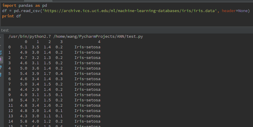
- 2、pandas: 直接处理和操作数据的主要package,提供了dataframe等方便处理表格数据的数据结构
安装如下:(pip方法)

import pandas as pd
df = pd.read_csv('https://archive.ics.uci.edu/ml/machine-learning-databases/iris/iris.data', header=None)
print df
- 3、statsmodels: 统计和计量经济学的package,包含了用于参数评估和统计测试的实用工具
-
 View Code
Python中的结构化数据分析利器-Pandas简介


17 September 2013
Pandas是python的一个数据分析包,最初由AQR Capital Management于2008年4月开发,并于2009年底开源出来,目前由专注于Python数据包开发的PyData开发team继续开发和维护,属于PyData项目的一部分。Pandas最初被作为金融数据分析工具而开发出来,因此,pandas为时间序列分析提供了很好的支持。 Pandas的名称来自于面板数据(panel data)和python数据分析(data analysis)。panel data是经济学中关于多维数据集的一个术语,在Pandas中也提供了panel的数据类型。 这篇文章会介绍一些Pandas的基本知识,偷了些懒其中采用的例子大部分会来自官方的10分钟学Pandas。我会加上个人的理解,帮助大家记忆和学习。

Pandas中的数据结构
Series:一维数组,与Numpy中的一维array类似。二者与Python基本的数据结构List也很相近,其区别是:List中的元素可以是不同的数据类型,而Array和Series中则只允许存储相同的数据类型,这样可以更有效的使用内存,提高运算效率。

Time- Series:以时间为索引的Series。

DataFrame:二维的表格型数据结构。很多功能与R中的data.frame类似。可以将DataFrame理解为Series的容器。以下的内容主要以DataFrame为主。

Panel :三维的数组,可以理解为DataFrame的容器。<!-- more -->

创建DataFrame
首先引入Pandas及Numpy:

import pandas as pd
import numpy as np
官方推荐的缩写形式为pd,你可以选择其他任意的名称。 DataFrame是二维的数据结构,其本质是Series的容器,因此,DataFrame可以包含一个索引以及与这些索引联合在一起的Series,由于一个Series中的数据类型是相同的,而不同Series的数据结构可以不同。因此对于DataFrame来说,每一列的数据结构都是相同的,而不同的列之间则可以是不同的数据结构。或者以数据库进行类比,DataFrame中的每一行是一个记录,名称为Index的一个元素,而每一列则为一个字段,是这个记录的一个属性。 创建DataFrame有多种方式:

以字典的字典或Series的字典的结构构建DataFrame,这时候的最外面字典对应的是DataFrame的列,内嵌的字典及Series则是其中每个值。
d = {'one' : pd.Series([1., 2., 3.], index=['a', 'b', 'c']),'two' : pd.Series([1., 2., 3., 4.], index=['a', 'b', 'c', 'd'])}
df = pd.DataFrame(d)
可以看到d是一个字典,其中one的值为Series有3个值,而two为Series有4个值。由d构建的为一个4行2列的DataFrame。其中one只有3个值,因此d行one列为NaN(Not a Number)--Pandas默认的缺失值标记。

从列表的字典构建DataFrame,其中嵌套的每个列表(List)代表的是一个列,字典的名字则是列标签。这里要注意的是每个列表中的元素数量应该相同。否则会报错:
ValueError: arrays must all be same length
从字典的列表构建DataFrame,其中每个字典代表的是每条记录(DataFrame中的一行),字典中每个值对应的是这条记录的相关属性。
d = [{'one' : 1,'two':1},{'one' : 2,'two' : 2},{'one' : 3,'two' : 3},{'two' : 4}]
df = pd.DataFrame(d,index=['a','b','c','d'],columns=['one','two'])
df.index.name='index'
以上的语句与以Series的字典形式创建的DataFrame相同,只是思路略有不同,一个是以列为单位构建,将所有记录的不同属性转化为多个Series,行标签冗余,另一个是以行为单位构建,将每条记录转化为一个字典,列标签冗余。使用这种方式,如果不通过columns指定列的顺序,那么列的顺序会是随机的。

个人经验是对于从一些已经结构化的数据转化为DataFrame似乎前者更方便,而对于一些需要自己结构化的数据(比如解析Log文件,特别是针对较大数据量时),似乎后者更方便。创建了DataFrame后可以通过index.name属性为DataFrame的索引指定名称。

DataFrame转换为其他类型
df.to_dict(outtype='dict')
outtype的参数为‘dict’、‘list’、‘series’和‘records’。 dict返回的是dict of dict;list返回的是列表的字典;series返回的是序列的字典;records返回的是字典的列表

查看数据
head和tail方法可以显示DataFrame前N条和后N条记录,N为对应的参数,默认值为5。这通常是拿到DataFrame后的第一个命令,可以方便的了解数据内容和含义。

df.head()
one    two
index
a    1    1
b    2    2
c    3    3
d    NaN    4
4 rows × 2 columns

R中的对应函数:

head(df)
df.tail()
one    two
index
a    1    1
b    2    2
c    3    3
d    NaN    4
4 rows × 2 columns

index(行)和columns(列)属性,可以获得DataFrame的行和列的标签。这也是了解数据内容和含义的重要步骤。

df.index
Index([u'a', u'b', u'c', u'd'], dtype='object')
查看字段名

df.columns
Index([u'one', u'two'], dtype='object')
decribe方法可以计算各个列的基本描述统计值。包含计数,平均数,标准差,最大值,最小值及4分位差。

df.describe()
one    two
count    3.0    4.000000
mean    2.0    2.500000
std    1.0    1.290994
min    1.0    1.000000
25%    1.5    1.750000
50%    2.0    2.500000
75%    2.5    3.250000
max    3.0    4.000000
8 rows × 2 columns

R中的对应函数:

summary(df)
行列转置
df.T
index    a    b    c    d
one    1    2    3    NaN
two    1    2    3    4
2 rows × 4 columns

排序
DataFrame提供了多种排序方式。

df.sort_index(axis=1, ascending=False)
sort_index可以以轴的标签进行排序。axis是指用于排序的轴,可选的值有0和1,默认为0即行标签(Y轴),1为按照列标签排序。 ascending是排序方式,默认为True即降序排列。

df.sort(columns='two')
df.sort(columns=['one','two'],ascending=[0,1])
DataFrame也提供按照指定列进行排序,可以仅指定一个列作为排序标准(以单独列名作为columns的参数),也可以进行多重排序(columns的参数为一个列名的List,列名的出现顺序决定排序中的优先级),在多重排序中ascending参数也为一个List,分别与columns中的List元素对应。

读写数据
DataFrame可以方便的读写数据文件,最常见的文件为CSV或Excel。Pandas读写Excel文件需要openpyxl(Excel 2007), xlrd/xlwt(Excel 2003)。

从CSV中读取数据:

df = pd.read_csv('foo.csv')
R中的对应函数:

df = read.csv('foo.csv')
将DataFrame写入CSV:

df.to_csv('foo.csv')
R中的对应函数:

df.to.csv('foo.csv')
从Excel中读取数据:

xls = ExcelFile('foo.xlsx')
xls.parse('sheet1', index_col=None, na_values=['NA'])
先定义一个Excel文件,用xls.parse解析sheet1的内容,index_col用于指定index列,na_values定义缺失值的标识。

将DataFrame写入Excel文件:

df.to_excel('foo.xlsx', sheet_name='sheet1')
默认的sheet为sheet1,也可以指定其他sheet名。

数据切片
通过下标选取数据:

df['one']
df.one
以上两个语句是等效的,都是返回df名称为one列的数据,返回的为一个Series。

df[0:3]
df[0]
下标索引选取的是DataFrame的记录,与List相同DataFrame的下标也是从0开始,区间索引的话,为一个左闭右开的区间,即[0:3]选取的为1-3三条记录。与此等价,还可以用起始的索引名称和结束索引名称选取数据:

df['a':'b']
有一点需要注意的是使用起始索引名称和结束索引名称时,也会包含结束索引的数据。以上两种方式返回的都是DataFrame。

使用标签选取数据:

df.loc[行标签,列标签]
df.loc['a':'b']#选取ab两行数据
df.loc[:,'one']#选取one列的数据
df.loc的第一个参数是行标签,第二个参数为列标签(可选参数,默认为所有列标签),两个参数既可以是列表也可以是单个字符,如果两个参数都为列表则返回的是DataFrame,否则,则为Series。

使用位置选取数据:

df.iloc[行位置,列位置]
df.iloc[1,1]#选取第二行,第二列的值,返回的为单个值
df.iloc[0,2],:]#选取第一行及第三行的数据
df.iloc[0:2,:]#选取第一行到第三行(不包含)的数据
df.iloc[:,1]#选取所有记录的第一列的值,返回的为一个Series
df.iloc[1,:]#选取第一行数据,返回的为一个Series
PS:loc为location的缩写,iloc则为integer & location的缩写

更广义的切片方式是使用.ix,它自动根据你给到的索引类型判断是使用位置还是标签进行切片

df.ix[1,1]
df.ix['a':'b']
通过逻辑指针进行数据切片:

df[逻辑条件]
df[df.one >= 2]#单个逻辑条件
df[(df.one >=1 ) & (df.one < 3) ]#多个逻辑条件组合
这种方式获得的数据切片都是DataFrame。

基本运算
Pandas支持基本的运算及向量化运算。

df.mean()#计算列的平均值,参数为轴,可选值为0或1.默认为0,即按照列运算
df.sum(1)#计算行的和
df.apply(lambda x: x.max() - x.min())#将一个函数应用到DataFrame的每一列,这里使用的是匿名lambda函数,与R中apply函数类似
设置索引
df.set_index('one')
重命名列
df.rename(columns={u'one':'1'}, inplace=True)
查看每个列的数据类型
df.dtypes
R中的对应函数:

str(df)
查看最大值/最小值
pd.Series.max()
pd.Series.idxmax()
重设索引
df.reset_index(inplace=True)
改变数据类型
df['A'].astype(float)
计算Series每个值的频率
df['A'].value_counts()
R的对应函数:

table(df['A'])
字符方法
pandas提供许多向量化的字符操作,你可以在str属性中找到它们

s.str.lower()
s.str.len()
s.str.contains(pattern)
DataFrame的合并
Contact:

ds = [{'one' : 4,'two':2},{'one' : 5,'two' : 3},{'one' : 6,'two' : 4},{'two' : 7,'three':10}]
dfs = pd.DataFrame(ds,index=['e','f','g','h'])
##构建一个新的DataFrame,dfs
df_t=pd.concat([df,dfs])#合并两个DataFrame
Merge(类似SQL中的Join操作):

left = pd.DataFrame({'key': ['foo1', 'foo2'], 'lval': [1, 2]})
right = pd.DataFrame({'key': ['foo1', 'foo2'], 'rval': [4, 5]})
#构建了两个DataFrame
pd.merge(left, right, on='key')#按照key列将两个DataFrame join在一起
DataFrame中的Group by:

df = pd.DataFrame({'A' : ['foo', 'bar', 'foo', 'bar','foo', 'bar', 'foo', 'foo'],
                    'B' : ['one', 'one', 'two', 'three','two', 'two', 'one', 'three'],
                    'C' :randn(8), 'D' : randn(8)});
df.groupby('A').sum()#按照A列的值分组求和
df.groupby(['A','B']).sum()##按照A、B两列的值分组求和
对应R函数:

tapply()
在实际应用中,先定义groups,然后再对不同的指标指定不同计算方式。

groups = df.groupby('A')#按照A列的值分组求和
groups['B'].sum()##按照A列的值分组求B组和
groups['B'].count()##按照A列的值分组B组计数
默认会以groupby的值作为索引,如果不将这些值作为索引,则需要使用as_index=False

df.groupby(['A','B'], as_index=False).sum()
构建透视表
使用pivot_table和crosstab都可以创建数据透视表

df = pd.DataFrame({'A' : ['one', 'one', 'two', 'three'] * 3,'B' : ['A', 'B', 'C'] * 4,
                'C' : ['foo', 'foo', 'foo', 'bar', 'bar', 'bar'] * 2,
                'D' : np.random.randn(12), 'E' : np.random.randn(12)})
pd.pivot_table(df, values = 'D', rows = ['A', 'B'], cols = ['C'])#以A、B为行标签,以C为列标签将D列的值汇总求和
pd.crosstab(rows = ['A', 'B'], cols = ['C'], values = 'D')#以A、B为行标签,以C为列标签将D列的值汇总求和
 时间序列分析
时间序列也是Pandas的一个特色。时间序列在Pandas中就是以Timestamp为索引的Series。

pandas提供to_datetime方法将代表时间的字符转化为Timestamp对象:

s = '2013-09-16 21:00:00'
ts = pd.to_datetime(s)
有时我们需要处理时区问题:

ts=pd.to_datetime(s,utc=True).tz_convert('Asia/Shanghai')
构建一个时间序列:

rng = pd.date_range('1/1/2012', periods=5, freq='M')
ts = pd.Series(randn(len(rng)), index=rng)
Pandas提供resample方法对时间序列的时间粒度进行调整:

ts_h=ts.resample('H', how='count')#M,5Min,1s
以上是将时间序列调整为小时,还可以支持月(M),分钟(Min)甚至秒(s)等。

画图
Pandas也支持一定的绘图功能,需要安装matplot模块。

比如前面创建的时间序列,通过plot()就可以绘制出折线图,也可以使用hist()命令绘制频率分布的直方图。

关于Panda作图,请查看另一篇博文:用Pandas作图

以上是关于Pandas的简单介绍,其实除了Pandas之外,Python还提供了多个科学计算包,比如Numpy,Scipy,以及数据挖掘的包:Scikit Learn,Orage,NLTK等,感兴趣的同学可以了解一下。

python 17
数据科学 3
dataframe 1
Pandas 2
数据分析 1
时间序列分析 1
- 4、matplotlib、pyplot、pylab: 用于生成统计图。pyplot 和 pylab属于matplotlib的子模块,所以只需安装matplotlib,就会有pyplot和pylab的了。(The difference between pylab and pyplot is that the former imports numpy into its namespace. This was to make it behave more similarly with matlab. Using pyplot instead of pylab is preferred now because it is cleaner. )

Python一般使用Matplotlib制作统计图形,用它自己的说法是‘让简单的事情简单,让复杂的事情变得可能’。(你说国外的“码农”咋这么会说,我就整不出来这工整的句子!)用它可以制作折线图,直方图,条形图,散点图,饼图,谱图等等你能想到的和想不到的统计图形,这些图形可以导出为多种具有出版质量的格式。此外,它和ipython结合使用,确实方便,谁用谁知道!
在Matplotlib里面经常使用到的是pylab和pyplot,它之间的区别在于pyplot是封装好的调用matplotlib底层制图库的接口,制图时用户不用关心底层的实现,而pylab则是为了使用者的方便,将numpy和pyplot的功能集中在了一个命名空间中。这么解释,可能还是不太清楚,因此在此次举个例子:
|
1
2
3
4
5
6
7
8
9
10
11
12
13
14
15
16
17
18
19
|
import pylabimport numpy as npimport matplotlib.pyplot as pltpylab.randn(2,3)array([[ 1.22356117, -0.62786477, -0.02927331],[ 1.11739661, -1.64112491, 2.24982297]])np.random.randn(2,3)array([[-1.41691502, -1.43500335, -0.68452086],[-0.53925581, -0.18478012, -0.0126745 ]])pylab.hist([1,1,1,2,3,3])plt.hist([1,1,1,2,3,3]) |
从上面的例子可以看在pylab中可以使用numpy中的一些方法,而在pyplot中不能使用numpy的方法;pylab和pyplot都可以制作统计图形。
- 5、libsvm:svm模型的一个库。附安装方法:
先从网站下载LibSVM的安装包(http://www.csie.ntu.edu.tw/~cjlin/cgi-bin/libsvm.cgi?+http://www.csie.ntu.edu.tw/~cjlin/libsvm+tar.gz),然后解压。
从终端进入解压目录,输入 make,例如我下载的是libsvm-3.20.tar.gz
cd /home/eple/Downloads/libsvm-3.20
make
然后进入python目录,同样输入make:(该步骤会生成 libsvm.so.2)
cd python/
make
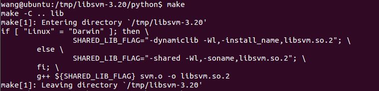
好了,搞定!为了测试是否成功,在终端启动python,输入:(附上官方提供的例子)
Quick Start
===========
There are two levels of usage. The high-level one uses utility functions
in svmutil.py and the usage is the same as the LIBSVM MATLAB interface.
>>> from svmutil import *
# Read data in LIBSVM format
>>> y, x = svm_read_problem('../heart_scale')
>>> m = svm_train(y[:200], x[:200], '-c 4')
>>> p_label, p_acc, p_val = svm_predict(y[200:], x[200:], m)
# Construct problem in python format
# Dense data
>>> y, x = [1,-1], [[1,0,1], [-1,0,-1]]
# Sparse data
>>> y, x = [1,-1], [{1:1, 3:1}, {1:-1,3:-1}]
>>> prob = svm_problem(y, x)
>>> param = svm_parameter('-t 0 -c 4 -b 1')
>>> m = svm_train(prob, param)
但是,要在Pycharm下,这样做还是不够的。还需要把 libsvm-3.18/python/*py文件放到 /usr/lib/python2.7/dist-packages 中, libsvm.so.2 放到 /usr/lib/python2.7/中
sudo cp *.py /usr/lib/python2.7/dist-packages
sudo cp /home/eple/Downloads/libsvm-3.20/libsvm.so.2 /usr/lib/python2.7
OK!
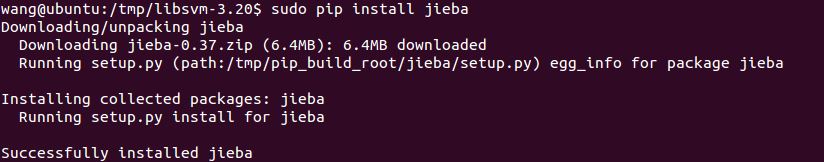
- 6、jieba:中文分词工具。附安装方法:
“结巴”中文分词:做最好的 Python 中文分词组件

"Jieba" (Chinese for "to stutter") Chinese text segmentation: built to be the best Python Chinese word segmentation module.

特点
    支持三种分词模式:

    精确模式,试图将句子最精确地切开,适合文本分析;
    全模式,把句子中所有的可以成词的词语都扫描出来, 速度非常快,但是不能解决歧义;
    搜索引擎模式,在精确模式的基础上,对长词再次切分,提高召回率,适合用于搜索引擎分词。
    支持繁体分词

    支持自定义词典
    MIT 授权协议
在线演示
    http://jiebademo.ap01.aws.af.cm/


网站代码:https://github.com/fxsjy/jiebademo

安装说明
    代码对 Python 2/3 均兼容

    全自动安装:easy_install jieba 或者 pip install jieba / pip3 install jieba
    半自动安装:先下载 http://pypi.python.org/pypi/jieba/ ,解压后运行 python     setup.py install
    手动安装:将 jieba 目录放置于当前目录或者 site-packages 目录
    通过 import jieba 来引用
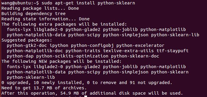
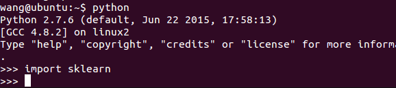
7、scikit-learn工具包:是一个基于SciPy和Numpy的开源机器学习模块,包括分类、回归、聚类系列算法,主要算法有SVM、逻辑回归、朴素贝叶斯、Kmeans、DBSCAN等;也提供了一些语料库。
[英文简介]Scikit-learn is a Python module integrating a wide range of state-of-the-art machine learning algorithms for medium-scale supervised and unsupervised problems. This package focuses on bringing machine learning to non-specialists using a general-purpose high-level language. Emphasis is put on ease of use, performance, documentation, and API consistency. It has minimal dependencies and is distributed under the simplified BSD license, encouraging its use in both academic and commercial settings. Source code, binaries, and documentation can be downloaded from http://scikit-learn.sourceforge.net.
项目主页:
https://pypi.python.org/pypi/scikit-learn/
https://github.com/scikit-learn/scikit-learn
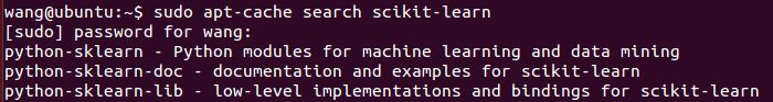
附安装方法1:
在Ubuntu源上可以直接找到该工具包,如下图:
直接安装:
附安装方法2:pip

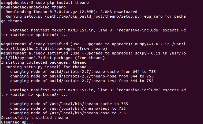
8、Theano深度学习
Theano是一个机器学习库,允许你定义、优化和评估涉及多维数组的数学表达式,这可能是其它库开发商的一个挫折点。与scikit-learn一样,Theano也很好地整合了NumPy库。GPU的透明使用使得Theano可以快速并且无错地设置,这对于那些初学者来说非常重要。然而有些人更多的是把它描述成一个研究工具,而不是当作产品来使用,因此要按需使用。
Theano最好的功能之一是拥有优秀的参考文档和大量的教程。事实上,多亏了此库的流行程度,使你在寻找资源的时候不会遇到太多的麻烦,比如如何得到你的模型以及运行等。
安装如下:
9、wikipedia :Wikipedia is a Python library that makes it easy to access and parse data from Wikipedia
Search Wikipedia, get article summaries, get data like links and images from a page, and more. Wikipedia wraps the MediaWiki APIso you can focus on using Wikipedia data, not getting it.
下面我说明在Ubuntu下的安装:


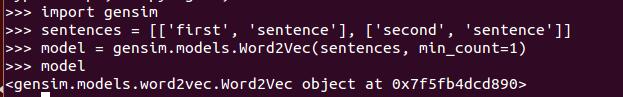
10、gensim:依赖NumPy和SciPy这两大Python科学计算工具包,一种简单的安装方法是pip install。gensim的这个官方安装页面很详细的列举了兼容的Python和NumPy, SciPy的版本号以及安装步骤,感兴趣的同学可以直接参考。下面我说明在Ubuntu下的安装:

11、Pattern (Github:http://github.com/clips/pattern)
此库更像是一个“全套”库,因为它不仅提供了一些机器学习算法,而且还提供了工具来帮助你收集和分析数据。数据挖掘部分可以帮助你收集来自谷歌、推特和维基百科等网络服务的数据。它也有一个Web爬虫和HTML DOM解析器。“引入这些工具的优点就是:在同一个程序中收集和训练数据显得更加容易。
在文档中有个很好的例子,使用一堆推文来训练一个分类器,用来区分一个推文是“win”还是“fail”。
 1 from pattern.web import Twitter
 2 from pattern.en import tag
 3 from pattern.vector import KNN, count
 4
 5 twitter, knn = Twitter(), KNN()
 6
 7 for i in range(1, 3):
 8     for tweet in twitter.search('#win OR #fail', start=i, count=100):
 9         s = tweet.text.lower()
10         p = '#win' in s and 'WIN' or 'FAIL'
11         v = tag(s)
12         v = [word for word, pos in v if pos == 'JJ'] # JJ = adjective
13         v = count(v) # {'sweet': 1}
14         if v:
15             knn.train(v, type=p)
16
17 print knn.classify('sweet potato burger')
18 print knn.classify('stupid autocorrect')
首先使用twitter.search()通过标签’#win’和’#fail’来收集推文数据。然后利用从推文中提取的形容词来训练一个K-近邻(KNN)模型。经过足够的训练,你会得到一个分类器。仅仅只需15行代码,还不错。
擅长:自然语言处理(NLP)和分类。
12、NLTK:Natural Language Toolkit
参考:
NLTK is a leading platform for building Python programs to work with human language data. It provides easy-to-use interfaces to over 50 corpora and lexical resources such as WordNet, along with a suite of text processing libraries for classification, tokenization, stemming, tagging, parsing, and semantic reasoning, wrappers for industrial-strength NLP libraries, and an active discussion forum.
NLTK has been called “a wonderful tool for teaching, and working in, computational linguistics using Python,” and “an amazing library to play with natural language.”
入门指导: Natural Language Processing with Python provides a practical introduction to programming for language processing. Written by the creators of NLTK, it guides the reader through the fundamentals of writing Python programs, working with corpora, categorizing text, analyzing linguistic structure, and more. The book is being updated for Python 3 and NLTK 3. (The original Python 2 version is still available at http://nltk.org/book_1ed.)
安装NLTK:
- Install NLTK: run
sudo pip install --user -U nltk - Install Numpy (optional): run
sudo pip install -U numpy - Test installation: run
pythonthen typeimport nltk
For older versions of Python it might be necessary to install setuptools (seehttp://pypi.python.org/pypi/setuptools) and to install pip (sudo easy_install pip).
安装NLTK语料:
因为标注数据等功能需要调用数据,所以需要下载NLTK数据包
For central installation on a multi-user machine, do the following from an administrator account.
Run the Python interpreter and type the commands:
>>> import nltk
>>> nltk.download()
A new window should open, showing the NLTK Downloader. Click on the File menu and select Change Download Directory. For central installation, set this to C:
ltk_data (Windows),/usr/local/share/nltk_data (Mac), or /usr/share/nltk_data (Unix). Next, select the packages or collections you want to download.
输入nltk.download()就会弹出窗口供选择,一般选择book可安装所有语料和包等:

Some simple things you can do with NLTK:
Tokenize and tag some text:
>>> import nltk
>>> sentence = """At eight o'clock on Thursday morning
... Arthur didn't feel very good."""
>>> tokens = nltk.word_tokenize(sentence)
>>> tokens
['At', 'eight', "o'clock", 'on', 'Thursday', 'morning',
'Arthur', 'did', "n't", 'feel', 'very', 'good', '.']
>>> tagged = nltk.pos_tag(tokens)
>>> tagged[0:6]
[('At', 'IN'), ('eight', 'CD'), ("o'clock", 'JJ'), ('on', 'IN'),
('Thursday', 'NNP'), ('morning', 'NN')]
Identify named entities:
>>> entities = nltk.chunk.ne_chunk(tagged)
>>> entities
Tree('S', [('At', 'IN'), ('eight', 'CD'), ("o'clock", 'JJ'),
           ('on', 'IN'), ('Thursday', 'NNP'), ('morning', 'NN'),
       Tree('PERSON', [('Arthur', 'NNP')]),
           ('did', 'VBD'), ("n't", 'RB'), ('feel', 'VB'),
           ('very', 'RB'), ('good', 'JJ'), ('.', '.')])
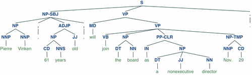
Display a parse tree:
>>> from nltk.corpus import treebank
>>> t = treebank.parsed_sents('wsj_0001.mrg')[0]
>>> t.draw()
NB. If you publish work that uses NLTK, please cite the NLTK book as follows:
Bird, Steven, Edward Loper and Ewan Klein (2009), Natural Language Processing with Python. O’Reilly Media Inc.