Abstract
Anomaly detection refers to the task of finding unusual instances that stand out from the normal data. In several applications, these outliers or anomalous instances are of greater interest compared to the normal ones. Specifically in the case of industrial optical inspection and infrastructure asset management, finding these defects (anomalous regions) is of extreme importance. Traditionally and even today this process has been carried out manually. Humans rely on the saliency of the defects in comparison to the normal texture to detect the defects. However, manual inspection is slow, tedious, subjective and susceptible to human biases. Therefore, the automation of defect detection is desirable. But for defect detection lack of availability of a large number of anomalous instances and labelled data is a problem. In this paper, we present a convolutional auto-encoder architecture for anomaly detection that is trained only on the defect-free (normal) instances. For the test images, residual masks that are obtained by subtracting the original image from the auto-encoder output are thresholded to obtain the defect segmentation masks. The approach was tested on two data-sets and achieved an impressive average F1 score of 0.885. The network learnt to detect the actual shape of the defects even though no defected images were used during the training.
摘要
异常检测是指从正常样本中发现异常实例的任务。在一些应用中,与正常值做对比,这些异常或者反常实例更加有意义。特别的,如工业光学检测的例子和基础设备资产管理,发现这些缺陷(异常区域)是非常重要的。传统的乃至今天这些流程还是用人工进行操作。人们依靠相比于正常细节的缺陷显著性来检测缺陷。然而,人工检测是缓慢的,冗长的,主观的,易受人类的偏见影响。因此,自动化的缺陷检测是令人向往的。但是在缺陷检测中, 缺乏大量的缺陷实例和标签数据是一个问题。在这篇文章中,我们提出一种卷积自动化编译结果对于缺陷检测,这个可以只使用正常样本进行训练。对于测试图片中,通过将原始的图片减去生成后的图片生成残差掩膜,通过阈值后,生成检测分割任务。这个方法在两个数据集上做测试并且实现了平均0.885的F1得分。这个网络学习去发现实际的缺陷,尽管在训练过程中没有缺陷图片。
Introduction
An anomaly is anything that deviates from the norm. Anomaly detection refers to the task of finding the anomalous instances. Defect detection is a special case of anomaly detection and has applications in industrial settings. Manual inspection by humans is still the norm in most of the industries. The inspection process iscompletely dependent on the visual difference of the anomaly (defect) from the normal background or texture. The process is prone to errors and has several drawbacks, such as training time and cost, human bias and subjectivity, among others. Individual factors such as age, visual acuity, scanning strategy, experience, and training impact the errors caused during the manual inspection process [1]. As a result of these challenges faced in the manual inspection by humans, automation of defect detection has been a topic of research across different application areas such as steel surfaces [2], rail tracks [3] and fabric [4], to name a few. However, all these techniques face two common problems: lack of large labelled data and the limited number of anomalous samples. Semi-supervised techniques try to tackle this challenge. These techniques are based on the assumption that we have access to the labels for only one class type i.e. the normal class [5]. They try to estimate the underlying distribution of the normal samples either implicitly or explicitly. This is followed by the measurement of deviation or divergence of the test samples from this distribution to determine an anomalous sample. To take an example of semi-supervised anomaly detection, Schlegl et al. [6] used Generative Adversarial Networks (GANs) for anomaly detection in optical coherence tomography images of the retina. They trained a GAN on the normal data to learn the underlying distribution of the anatomical variability. But they did not train an encoder for mapping the input image to the latent space. Because of this, the method needed an optimization step for every test image to find a point in the latent space that corresponded to the most visually similar generated image which made it slow. In this research, we explore an auto-encoder based approach that also tries to estimate the distribution of the normal data and then uses residual maps to find the defects. It is described in the next section
简介
异常是指任何偏离正常的东西. 异常检测是指发现异常实例化的任务。缺陷检测是一个特殊的异常检测而且在工业上有应用。人工检视在工业应用上仍然是常见的。这个检视的过程依赖于正常背景和纹理与异常(缺陷)的视觉不同。其他的,工业因素比如年龄,视力灵敏度,扫描策略,经验,培训影响了在人工检测上错误的发生。由于这些挑战面临着人工检查,自动的缺陷检测依据是一个顶尖的研究在不同应用领域如钢材表面,轨道和布料。举几个例子,然而,所有的技术面临这两个共同的问题: 缺少大量的标记数据以及有限的缺陷样本。半监督技术尝试去处理这个挑战。这些技术都是假定我们可以访问一个类类型的标签,及普通类。他们尝试去评估正态样本的潜在分布或潜或显。以半监督异常检测为例, Schlegl et al使用对抗生成网络针对异常检测在光学相干层析成像中的视网膜图像。他们训练一个Gan在通常数据上去学习解剖变异的潜在分布。但是他们没有训练一个编码器去映射一个输入图片转换为潜在空间。因为这样,这个方法需要一个优化步骤对于每一张测试图片在潜在空间上发现一个点,并且与视觉上最相似的生成图片,这使得它变慢。在这个研究中,我们采用了一个基于方法的自动编码器,这个方法可以评估正常数据的分布,并且使用残差图去发现这些缺陷,这将在下一节做解释。
本文的关键优化点:
1. 通过auto-encode网络,输入是正常的图片,输出也是预测图片,与输入图片构成MSE LOSS, 因为网络没有学习到缺陷的样子,因此当缺陷图片输入的时候,预测的结果无法生成有缺陷的位置,因此缺陷图片减去预测图片,结果就是缺陷的位置信息。
Method
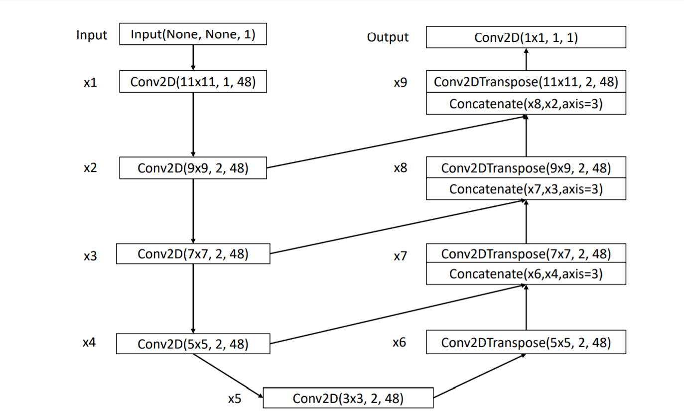
The proposed network architecture is shown in Figure 1. It is similar to the UNet [7] architecture. The encoder (layers x1 to x5) uses progressively decreasing filter sizes from 11×11 to 3×3. This decreasing filter size is chosen to allow for a larger field of view for the network without having to use large number of smaller size filters. Since deeper networks have a greater tendency to over-fit to the data and have poor generalization. The decoder structure has kernel sizes that are in the reverse of the encoder order and uses Transposed Convolution Layers. The output from the encoder layers is concatenated with the previous layers before passing to layers x7 to x9. For every Conv2D(Transpose) layer the parameters shown are kernel size, stride and number of filters for that layer. After every layer, batch normalization [8] is applied which is followed by the ReLU activation function [9]. For a H ×W input the network outputs a H ×W reconstruction. The network is trained on only the defect-free or normal data samples. Tensorflow 2.0 was used for conducting the experiments. The loss function used was the L2 norm or MSE (Mean Squared Error). The label in this case is the original input image and the prediction is the image reconstructed by the auto-encoder. Adam optimizer [10] was used with default settings. The training was done for 50 epochs.
方法
提出的网络结构在第一张图上显示. 这与UNet的网络很像,编码器使用逐步的递减核大小从11x11到3x3. 这个递减的过滤器大小可以在网络中获得更大的感受眼而不需要使用更多的小尺寸的过滤器。因为更深的网络对于数据集更容易过拟合并且缺乏通用性。这个解码器结构与编码器有着相反的核尺寸并且使用转置卷积。编码器的输出在传递到X7和X9的时候与之前的层做连接。每一个Conv2D(转置)层的参数表示内核的尺寸,该层的步长和过滤器的个数。在接下来的每个层, 归一化层被应用在激活层函数之后。对于HxW的输出网络的输出一个HxW的重构。这个网络的训练只在没有缺陷或者普通数据样本上。Tensorflow2.0被用来指导这个实验。这个损失函数使用L2归一化或者平均方差损失。本例的输入在本例中是原始的输入图片,预测是通过自动编码的重构图片。使用Adam作为默认的设计,训练经过了50个epoch。
Our hypothesis is that the auto-encoder will learn representations that would only be able to encode and decode the normal samples properly and will not be able to reconstruct the anomalous regions. This shall cause large residuals for the defective regions in the residual map obtained by subtracting the reconstructed image from the input image as shown in Equation 1. The subtraction is done at per pixel-level. This is followed by a thresholding operation to obtain the final defect segmentation.
![]()
where R is the residual, X is the input and AE(X) is the output (reconstructed image) of the auto-encoder. The data-sets used for conducting the experiments are described next.
我们的假设是自动编码将会学习特征这个只能适用在正常图片的编解码上并且不能够被用来重建缺陷的区域。在残差图上,这造成了缺陷部位大面积的残余,通过输入图和重建图相减的结果在Equation 1. 这个相减针对每一个像素值。通过阈值的操作收集到最终的缺陷区域
这里R是残差,X是输入和AE(x)是自动编解码的输出(重构图像)。接下来将描述用于进行试验的数据集。
上述算法网络的代码:
class AnomalyAE(nn.Module):
    def __init__(self):
        super().__init__()
        self.conv1 = nn.Conv2d(1, 48, (11, 11), stride=(1, 1), padding=5)
        self.bn1 = nn.BatchNorm2d(48)

        self.conv2 = nn.Conv2d(48, 48, (9, 9), stride=(2, 2), padding=4)
        self.bn2 = nn.BatchNorm2d(48)

        self.conv3 = nn.Conv2d(48, 48, (7, 7), stride=(2, 2), padding=3)
        self.bn3 = nn.BatchNorm2d(48)

        self.conv4 = nn.Conv2d(48, 48, (5, 5), stride=(2, 2), padding=2)
        self.bn4 = nn.BatchNorm2d(48)

        self.conv5 = nn.Conv2d(48, 48, (3, 3), stride=(2, 2), padding=1)
        self.bn5 = nn.BatchNorm2d(48)

        self.conv_tr1 = nn.ConvTranspose2d(
            48, 48, (5, 5), stride=(2, 2), padding=2, output_padding=1)
        self.bn_tr1 = nn.BatchNorm2d(48)

        self.conv_tr2 = nn.ConvTranspose2d(
            96, 48, (7, 7), stride=(2, 2), padding=3, output_padding=1)
        self.bn_tr2 = nn.BatchNorm2d(48)

        sself.conv_tr3 = nn.ConvTranspose2d(
            96, 48, (9, 9), stride=(2, 2), padding=4, output_padding=1)
        self.bn_tr3 = nn.BatchNorm2d(48)

         self.conv_tr4 = nn.ConvTranspose2d(
            96, 48, (11, 11), stride=(2, 2), padding=5, output_padding=1)
        self.bn_tr4 = nn.BatchNorm2d(48)

        self.conv_output = nn.Conv2d(96, 1, (1, 1), (1, 1))
        self.bn_output = nn.BatchNorm2d(1)

 def forward(self, x):
        slope = 0.2
        x = F.leaky_relu((self.bn1(self.conv1(x))), slope)
        x1 = F.leaky_relu((self.bn2(self.conv2(x))), slope)
        x2 = F.leaky_relu((self.bn3(self.conv3(x1))), slope)
        x3 = F.leaky_relu((self.bn4(self.conv4(x2))), slope)
        x4 = F.leaky_relu((self.bn5(self.conv5(x3))), slope)

        x5 = F.leaky_relu(self.bn_tr1(self.conv_tr1(x4)), slope)
        x6 = F.leaky_relu(self.bn_tr2(
            self.conv_tr2(torch.cat([x5, x3], 1))), slope)
        x7 = F.leaky_relu(self.bn_tr3(
            self.conv_tr3(torch.cat([x6, x2], 1))), slope)
        x8 = F.leaky_relu(self.bn_tr4(
            self.conv_tr4(torch.cat([x7, x1], 1))), slope)

        output = F.leaky_relu(self.bn_output(
            self.conv_output(torch.cat([x8, x], 1))), slope)
        return output
上述的损失函数使用的是MSE loss
loss = F.mse_loss