数据可视化基础专题（十三）：Matplotlib 基础（五）常用图表（三）环形图、热力图、直方图

环形图

环形图其实是另一种饼图，使用的还是上面的 pie() 这个方法，这里只需要设置一下参数 wedgeprops 即可。

例子一：

import matplotlib.pyplot as plt

# 中文和负号的正常显示
plt.rcParams['font.sans-serif']=['SimHei']
plt.rcParams['axes.unicode_minus'] = False

# 数据
edu = [0.2515,0.3724,0.3336,0.0368,0.0057]
labels = ['中专','大专','本科','硕士','其他']

# 让本科学历离圆心远一点
explode = [0,0,0.1,0,0]

# 将横、纵坐标轴标准化处理，保证饼图是一个正圆，否则为椭圆
plt.axes(aspect='equal')

# 自定义颜色
colors=['#9999ff','#ff9999','#7777aa','#2442aa','#dd5555'] # 自定义颜色

# 绘制饼图
plt.pie(x=edu,  # 绘图数据
    explode = explode,  # 突出显示大专人群
    labels = labels,  # 添加教育水平标签
    colors = colors,  # 设置饼图的自定义填充色
    autopct = '%.1f%%',  # 设置百分比的格式，这里保留一位小数
    wedgeprops = {'width': 0.3, 'edgecolor':'green'}
    )

# 添加图标题
plt.title('xxx 公司员工教育水平分布')

# 保存图形
plt.savefig('pie_demo1.png')

这个示例仅仅在前面示例的基础上增加了一个参数 wedgeprops 的设置，我们看下结果：

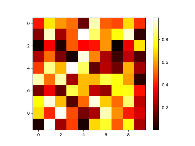
热力图

plt.imshow(x, cmap)

import numpy as np
import matplotlib.pyplot as plt

x = np.random.rand(10, 10)
plt.imshow(x, cmap=plt.cm.hot)

# 显示右边颜色条
plt.colorbar()

plt.savefig('imshow_demo.png')

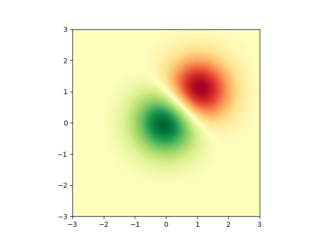
例子二

import numpy as np
import matplotlib.cm as cm
import matplotlib.pyplot as plt
import matplotlib.cbook as cbook
from matplotlib.path import Path
from matplotlib.patches import PathPatch

delta = 0.025
x = y = np.arange(-3.0, 3.0, delta)
X, Y = np.meshgrid(x, y)
Z1 = np.exp(-X**2 - Y**2)
Z2 = np.exp(-(X - 1)**2 - (Y - 1)**2)
Z = (Z1 - Z2) * 2

fig, ax = plt.subplots()
im = ax.imshow(Z, interpolation='bilinear', cmap=cm.RdYlGn,
               origin='lower', extent=[-3, 3, -3, 3],
               vmax=abs(Z).max(), vmin=-abs(Z).max())

plt.show()

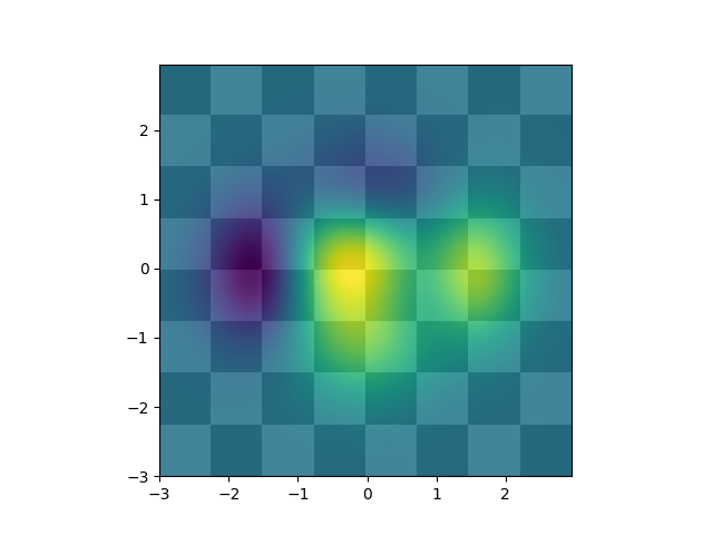
 例子3

import matplotlib.pyplot as plt
import numpy as np


def func3(x, y):
    return (1 - x / 2 + x**5 + y**3) * np.exp(-(x**2 + y**2))


# make these smaller to increase the resolution
dx, dy = 0.05, 0.05

x = np.arange(-3.0, 3.0, dx)
y = np.arange(-3.0, 3.0, dy)
X, Y = np.meshgrid(x, y)

# when layering multiple images, the images need to have the same
# extent.  This does not mean they need to have the same shape, but
# they both need to render to the same coordinate system determined by
# xmin, xmax, ymin, ymax.  Note if you use different interpolations
# for the images their apparent extent could be different due to
# interpolation edge effects

extent = np.min(x), np.max(x), np.min(y), np.max(y)
fig = plt.figure(frameon=False)

Z1 = np.add.outer(range(8), range(8)) % 2  # chessboard
im1 = plt.imshow(Z1, cmap=plt.cm.gray, interpolation='nearest',
                 extent=extent)

Z2 = func3(X, Y)

im2 = plt.imshow(Z2, cmap=plt.cm.viridis, alpha=.9, interpolation='bilinear',
                 extent=extent)

plt.show()

直方图

例子1

import matplotlib.pyplot as plt
import numpy as np
from matplotlib import colors
from matplotlib.ticker import PercentFormatter

# Fixing random state for reproducibility
np.random.seed(19680801)

N_points = 100000
n_bins = 20

# Generate a normal distribution, center at x=0 and y=5
x = np.random.randn(N_points)
y = .4 * x + np.random.randn(100000) + 5

fig, axs = plt.subplots(1, 2, sharey=True, tight_layout=True)

# We can set the number of bins with the `bins` kwarg
axs[0].hist(x, bins=n_bins)
axs[1].hist(y, bins=n_bins)

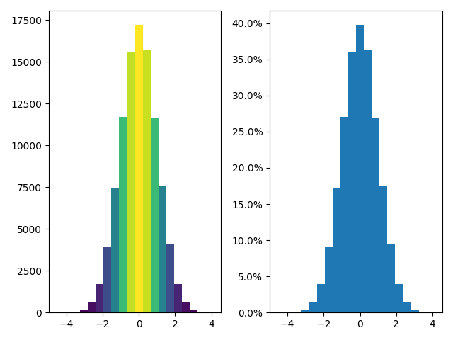
 例子2

fig, axs = plt.subplots(1, 2, tight_layout=True)

# N is the count in each bin, bins is the lower-limit of the bin
N, bins, patches = axs[0].hist(x, bins=n_bins)

# We'll color code by height, but you could use any scalar
fracs = N / N.max()

# we need to normalize the data to 0..1 for the full range of the colormap
norm = colors.Normalize(fracs.min(), fracs.max())

# Now, we'll loop through our objects and set the color of each accordingly
for thisfrac, thispatch in zip(fracs, patches):
    color = plt.cm.viridis(norm(thisfrac))
    thispatch.set_facecolor(color)

# We can also normalize our inputs by the total number of counts
axs[1].hist(x, bins=n_bins, density=True)

# Now we format the y-axis to display percentage
axs[1].yaxis.set_major_formatter(PercentFormatter(xmax=1))