神经网络，神经网络模型

概述

以监督学习为例，假设我们有训练样本集(x(i),y(i)),那么神经网络算法能够提供一种复杂且非线性的的假设模型h_w,b(x),它具有参数W，b，可以以此参数来拟合我们的数据。

为了描述神经网络，我们先从最简单的神经网络讲起，这个神经网络仅由一个“神经元”构成，以下即是这个神经元的图示：

这个“神经元”是一个以x_1,x₂,x₃及截距+1为输入值的运算单元，其输出为

其中函数 被称为“激活函数”。在本教程中，我们选择sigmoid函数作为激活函数f(.)                      

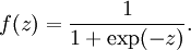
可以看出，这个单一“神经元”的输入——输出映射关系其实就是一个逻辑回归（logistic regression）.

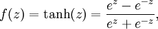
虽然本系列教程采用sigmoid函数，但你也可以选择双曲正切函数（tanh）:

以下分别是sigmoid及tanh的函数图像

函数是sigmoid函数的一种变体，它的取值范围为 ，而不是sigmoid函数的 。

最后要说明的是，有一个等式我们以后会经常用到：如果选择 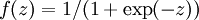，也就是sigmoid函数，那么它的导数就是 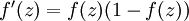（如果选择tanh函数，那它的导数就是 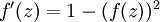，你可以根据sigmoid（或tanh）函数的定义自行推导这个等式。

神经网络模型

所谓神经网络就是将许多个单一“神经元”联结在一起，这样，一个“神经元”的输出就可以是另一个“神经元”的输入。例如，下图就是一个简单的神经网络：

我们使用圆圈来表示神经网络的输入，标上“”的圆圈被称为偏置节点，也就是截距项。神经网络最左边的一层叫做输入层，最右的一层叫做输出层（本例中，输出层只有一个节点）。中间所有节点组成的一层叫做隐藏层，因为我们不能在训练样本集中观测到它们的值。同时可以看到，以上神经网络的例子中有3个输入单元（偏置单元不计在内），3个隐藏单元及一个输出单元。

     我们用 来表示网络的层数，本例中 ，我们将第 层记为 ，于是 是输入层，输出层是 。

     本例神经网络有参数 ，其中 （下面的式子中用到）是第 层第 单元与第 层第 单元之间的联接参数（其实就是连接线上的权重，注意标号顺序）， 是第 层第 单元的偏置项。因此在本例中， ， 。

     注意：没有其他单元连向偏置单元（即偏置单元没有输入），因为它们总是输出+1.同时。同时，我们用 表示第 层的节点数（偏置单元不计在内）。

     我们用 表示第 层第 单元的激活值（输出值）。当 时， ，也就是第 个输入值（输入值的第 个特征）。对于给定参数集合 ，我们的神经网络就可以按照函数 来计算输出结果。本例神经网络的计算步骤如下：

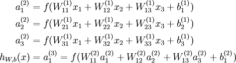
我们用 表示第 层第 单元输入加权和（包括偏置单元），比如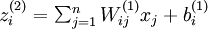， ，则 。 。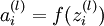

这样我们就可以得到一种更简洁的表示法。这里我们将激活函数f(.)扩展为用向量（分量的形式）来表示，即 ，那么，上面的等式可以更简洁地表示为：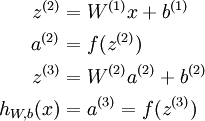

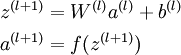
我们将上面的计算步骤叫作前向传播。回想一下，之前我们用 表示输入层的激活值，那么给定第 层的激活值 后，第 层的激活值 就可以按照下面步骤计算得到：

将参数矩阵化，使用矩阵－向量运算方式，我们就可以利用线性代数的优势对神经网络进行快速求解。 

 目前为止，我们讨论了一种神经网络，我们也可以构建另一种结构的神经网络（这里结构指的是神经元之间的联结模式），也就是包含多个隐藏层的神经网络。最常见的一个例子是 层的神经网络，第 层是输入层，第 层是输出层，中间的每个层 与层 紧密相联。这种模式下，要计算神经网络的输出结果，我们可以按照之前描述的等式，按部就班，进行前向传播，逐一计算第 层的所有激活值，然后是第 层的激活值，以此类推，直到第 层。这是一个前馈神经网络的例子，因为这种联接图没有闭环或回路。

 神经网络也可以有多个输出单元。比如，下面的神经网络有两个隐藏层： 及 ，输出层 有两个输出单元。

要求解这样的神经网络，需要样本集 ，其中 。如果你想预测的输出是多个的，那这种神经网络很适用。（比如，在医疗诊断应用中，患者的体征指标就可以作为向量的输入值，而不同的输出值 可以表示不同的疾病存在与否。）

 

中英文对照：

neural networks 神经网络

activation function 激活函数

hyperbolic tangent 双曲正切函数

bias units 偏置项

activation 激活值

forward propagation 前向传播

feedforward neural network 前馈神经网络