第七章、支持向量机SVM(非线性)
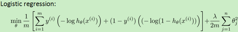
1.逻辑回归支持向量机
代价函数:
用cost1(z)代替![]() ,cost0(z)代替
,cost0(z)代替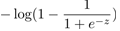 ,两个函数的图像:
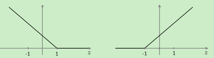
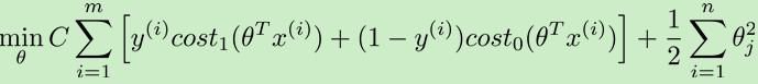
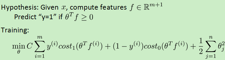
去掉m,用C代替lambda,得支持向量机的算法:
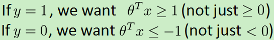
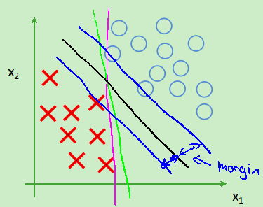
支持向量机的间距(大间隔分类):因为theta' *X>=1而不是0,所以会选择一条离数据最远的一条线,如图:会选择那条黑线
2.支持向量机能实现大间隔分类的原因:
设Ax+By=0表示一条线段,则(A,B)可以表示一条向量,并且和直线垂直。向量相乘可以等化为投影(有正负)乘以向量长度。p(i)表示X(i)在theta上的投影。原式可以转化为如下:
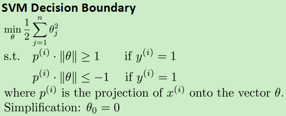
所以会尽可能让p(i)大,就会实现大间隔分类。
3.核函数kernel:处理更加复杂的非线性问题
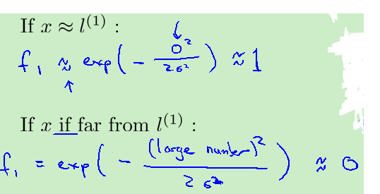
对每一个数据做一个等价代换:
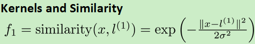
核函数性质:
![]() 的影响:越大越平缓
的影响:越大越平缓
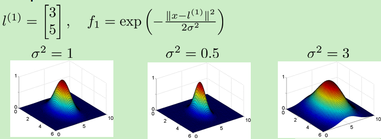
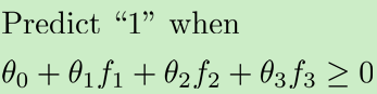
预测函数:
对于一个问题,![]() ?
?
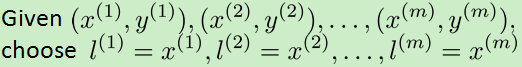
用每个数据集:
支持向量机的核函数求theta的h函数和cost函数:
注意上图中的正则化项在支持向量机中一般用theta' *m*theta(m为数据集个数),目的是提高效率。
4.支持向量机的核函数的高偏差和高方差:
C较大:低偏差高方差
C较小:高偏差低方差![]() 较大:图像较平缓,高偏差低方差
较大:图像较平缓,高偏差低方差![]() 较小:图像较陡峭,低偏差高方差
较小:图像较陡峭,低偏差高方差
5.在octave中使用自带的支持向量机的函数,需要提供一个函数实现(核函数):

在使用高斯函数前,一定要归一化,否则差距太大,可能会忽略掉小的特征值。
6.多分类:一对多,选最大的,和逻辑回归类似。
7.分类问题的选择
- 如果特征n相比数据集m较大,则一般不需要非常复杂的边界,用支持向量机的线性核函数(不使用核函数)或逻辑回归来形成一个简单地边界(大约:n=10000,m=10-1000)
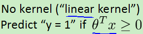
- 相反如果数据集较多,则想要一个较为复杂曲线的边界,用前面提到的支持向量机的高斯核函数(大约:n=1-1000,m=10-10000)

- 当m太大时,高斯核函数运行会很慢,一般会手动增加特征,并用线性核函数(不使用核函数)或逻辑回归来处理(m=50000+)
- 神经网络求解也很慢,优化的SVM会比它快,并且存在局部最优解而非整体最优解,能处理非常复杂的问题。
代码段1:支持向量机的线性核函数和高斯核函数(不是自己写的)mlclass-ex6-007
1.线性核函数
function sim = linearKernel(x1, x2)
    x1 = x1(:); x2 = x2(:);
    sim = x1' * x2;  % 不知道为什么?

end
2.高斯核函数
function sim = gaussianKernel(x1, x2, sigma)
    x1 = x1(:); x2 = x2(:);
    sim = 0;
    x=x1-x2;
    sim=exp(-(x' * x)/(2*sigma*sigma) );

end
3.高斯核函数选取![]() 和C
和C
function [C, sigma] = dataset3Params(X, y, Xval, yval)
    C = 1;
    sigma = 0.3;
        value=[0.01 0.03 0.1 0.3 1 3 10 30]';
    error=2;

    for i=1:size(value,1)
        tC=value(i);
        for j=1:size(value,1)
            tsigma=value(j);
            model= svmTrain(X, y, tC, @(x1, x2) gaussianKernel(x1, x2, tsigma)); %支持向量机算法
            predictions = svmPredict(model, Xval);    %支持向量机预测算法
            terror=mean(double(predictions ~= yval));
            if terror<error
                error=terror;
                C=tC;
                sigma=tsigma;
            end;
        end;
    end;
end
4.svmTrain,visualizeBoundaryLinear,visualizeBoundary,svmPredict(自带)


function [model] = svmTrain(X, Y, C, kernelFunction, ...
                            tol, max_passes)
%SVMTRAIN Trains an SVM classifier using a simplified version of the SMO
%algorithm.
%   [model] = SVMTRAIN(X, Y, C, kernelFunction, tol, max_passes) trains an
%   SVM classifier and returns trained model. X is the matrix of training
%   examples.  Each row is a training example, and the jth column holds the
%   jth feature.  Y is a column matrix containing 1 for positive examples
%   and 0 for negative examples.  C is the standard SVM regularization
%   parameter.  tol is a tolerance value used for determining equality of
%   floating point numbers. max_passes controls the number of iterations
%   over the dataset (without changes to alpha) before the algorithm quits.
%
% Note: This is a simplified version of the SMO algorithm for training
%       SVMs. In practice, if you want to train an SVM classifier, we
%       recommend using an optimized package such as:
%
%           LIBSVM   (http://www.csie.ntu.edu.tw/~cjlin/libsvm/)
%           SVMLight (http://svmlight.joachims.org/)
%
%

if ~exist('tol', 'var') || isempty(tol)
    tol = 1e-3;
end

if ~exist('max_passes', 'var') || isempty(max_passes)
    max_passes = 5;
end

% Data parameters
m = size(X, 1);
n = size(X, 2);

% Map 0 to -1
Y(Y==0) = -1;

% Variables
alphas = zeros(m, 1);
b = 0;
E = zeros(m, 1);
passes = 0;
eta = 0;
L = 0;
H = 0;

% Pre-compute the Kernel Matrix since our dataset is small
% (in practice, optimized SVM packages that handle large datasets
%  gracefully will _not_ do this)
%
% We have implemented optimized vectorized version of the Kernels here so
% that the svm training will run faster.
if strcmp(func2str(kernelFunction), 'linearKernel')
    % Vectorized computation for the Linear Kernel
    % This is equivalent to computing the kernel on every pair of examples
    K = X*X';
elseif strfind(func2str(kernelFunction), 'gaussianKernel')
    % Vectorized RBF Kernel
    % This is equivalent to computing the kernel on every pair of examples
    X2 = sum(X.^2, 2);
    K = bsxfun(@plus, X2, bsxfun(@plus, X2', - 2 * (X * X')));
    K = kernelFunction(1, 0) .^ K;
else
    % Pre-compute the Kernel Matrix
    % The following can be slow due to the lack of vectorization
    K = zeros(m);
    for i = 1:m
        for j = i:m
             K(i,j) = kernelFunction(X(i,:)', X(j,:)');
             K(j,i) = K(i,j); %the matrix is symmetric
        end
    end
end

% Train
fprintf('
Training ...');
dots = 12;
while passes < max_passes,

    num_changed_alphas = 0;
    for i = 1:m,

        % Calculate Ei = f(x(i)) - y(i) using (2).
        % E(i) = b + sum (X(i, :) * (repmat(alphas.*Y,1,n).*X)') - Y(i);
        E(i) = b + sum (alphas.*Y.*K(:,i)) - Y(i);

        if ((Y(i)*E(i) < -tol && alphas(i) < C) || (Y(i)*E(i) > tol && alphas(i) > 0)),

            % In practice, there are many heuristics one can use to select
            % the i and j. In this simplified code, we select them randomly.
            j = ceil(m * rand());
            while j == i,  % Make sure i
eq j
                j = ceil(m * rand());
            end

            % Calculate Ej = f(x(j)) - y(j) using (2).
            E(j) = b + sum (alphas.*Y.*K(:,j)) - Y(j);

            % Save old alphas
            alpha_i_old = alphas(i);
            alpha_j_old = alphas(j);

            % Compute L and H by (10) or (11).
            if (Y(i) == Y(j)),
                L = max(0, alphas(j) + alphas(i) - C);
                H = min(C, alphas(j) + alphas(i));
            else
                L = max(0, alphas(j) - alphas(i));
                H = min(C, C + alphas(j) - alphas(i));
            end

            if (L == H),
                % continue to next i.
                continue;
            end

            % Compute eta by (14).
            eta = 2 * K(i,j) - K(i,i) - K(j,j);
            if (eta >= 0),
                % continue to next i.
                continue;
            end

            % Compute and clip new value for alpha j using (12) and (15).
            alphas(j) = alphas(j) - (Y(j) * (E(i) - E(j))) / eta;

            % Clip
            alphas(j) = min (H, alphas(j));
            alphas(j) = max (L, alphas(j));

            % Check if change in alpha is significant
            if (abs(alphas(j) - alpha_j_old) < tol),
                % continue to next i.
                % replace anyway
                alphas(j) = alpha_j_old;
                continue;
            end

            % Determine value for alpha i using (16).
            alphas(i) = alphas(i) + Y(i)*Y(j)*(alpha_j_old - alphas(j));

            % Compute b1 and b2 using (17) and (18) respectively.
            b1 = b - E(i) ...
                 - Y(i) * (alphas(i) - alpha_i_old) *  K(i,j)' ...
                 - Y(j) * (alphas(j) - alpha_j_old) *  K(i,j)';
            b2 = b - E(j) ...
                 - Y(i) * (alphas(i) - alpha_i_old) *  K(i,j)' ...
                 - Y(j) * (alphas(j) - alpha_j_old) *  K(j,j)';

            % Compute b by (19).
            if (0 < alphas(i) && alphas(i) < C),
                b = b1;
            elseif (0 < alphas(j) && alphas(j) < C),
                b = b2;
            else
                b = (b1+b2)/2;
            end

            num_changed_alphas = num_changed_alphas + 1;

        end

    end

    if (num_changed_alphas == 0),
        passes = passes + 1;
    else
        passes = 0;
    end

    fprintf('.');
    dots = dots + 1;
    if dots > 78
        dots = 0;
        fprintf('
');
    end
    if exist('OCTAVE_VERSION')
        fflush(stdout);
    end
end
fprintf(' Done!

');

% Save the model
idx = alphas > 0;
model.X= X(idx,:);
model.y= Y(idx);
model.kernelFunction = kernelFunction;
model.b= b;
model.alphas= alphas(idx);
model.w = ((alphas.*Y)'*X)';

end
function visualizeBoundaryLinear(X, y, model)
%VISUALIZEBOUNDARYLINEAR plots a linear decision boundary learned by the
%SVM
%   VISUALIZEBOUNDARYLINEAR(X, y, model) plots a linear decision boundary
%   learned by the SVM and overlays the data on it

    w = model.w;
    b = model.b;
    xp = linspace(min(X(:,1)), max(X(:,1)), 100);
    yp = - (w(1)*xp + b)/w(2);
    plotData(X, y);
    hold on;
    plot(xp, yp, '-b');
    hold off

end
function visualizeBoundary(X, y, model, varargin)
%VISUALIZEBOUNDARY plots a non-linear decision boundary learned by the SVM
%   VISUALIZEBOUNDARYLINEAR(X, y, model) plots a non-linear decision
%   boundary learned by the SVM and overlays the data on it

% Plot the training data on top of the boundary
    plotData(X, y)

    % Make classification predictions over a grid of values
    x1plot = linspace(min(X(:,1)), max(X(:,1)), 100)';
    x2plot = linspace(min(X(:,2)), max(X(:,2)), 100)';
    [X1, X2] = meshgrid(x1plot, x2plot);
    vals = zeros(size(X1));
    for i = 1:size(X1, 2)
       this_X = [X1(:, i), X2(:, i)];
       vals(:, i) = svmPredict(model, this_X);
    end

    % Plot the SVM boundary
    hold on
    contour(X1, X2, vals, [0 0], 'Color', 'b');
    hold off;

end
function pred = svmPredict(model, X)
%SVMPREDICT returns a vector of predictions using a trained SVM model
%(svmTrain).
%   pred = SVMPREDICT(model, X) returns a vector of predictions using a
%   trained SVM model (svmTrain). X is a mxn matrix where there each
%   example is a row. model is a svm model returned from svmTrain.
%   predictions pred is a m x 1 column of predictions of {0, 1} values.
%

% Check if we are getting a column vector, if so, then assume that we only
% need to do prediction for a single example
if (size(X, 2) == 1)
    % Examples should be in rows
    X = X';
end

% Dataset
m = size(X, 1);
p = zeros(m, 1);
pred = zeros(m, 1);

if strcmp(func2str(model.kernelFunction), 'linearKernel')
    % We can use the weights and bias directly if working with the
    % linear kernel
    p = X * model.w + model.b;
elseif strfind(func2str(model.kernelFunction), 'gaussianKernel')
    % Vectorized RBF Kernel
    % This is equivalent to computing the kernel on every pair of examples
    X1 = sum(X.^2, 2);
    X2 = sum(model.X.^2, 2)';
    K = bsxfun(@plus, X1, bsxfun(@plus, X2, - 2 * X * model.X'));
    K = model.kernelFunction(1, 0) .^ K;
    K = bsxfun(@times, model.y', K);
    K = bsxfun(@times, model.alphas', K);
    p = sum(K, 2);
else
    % Other Non-linear kernel
    for i = 1:m
        prediction = 0;
        for j = 1:size(model.X, 1)
            prediction = prediction + ...
                model.alphas(j) * model.y(j) * ...
                model.kernelFunction(X(i,:)', model.X(j,:)');
        end
        p(i) = prediction + model.b;
    end
end

% Convert predictions into 0 / 1
pred(p >= 0) =  1;
pred(p <  0) =  0;

end
5.整体代码
clear ; close all; clc
load('ex6data1.mat');

% Plot training data
%plotData(X, y);

%C = 10;
%model = svmTrain(X, y, C, @linearKernel, 1e-3, 20);
%visualizeBoundaryLinear(X, y, model);

x1 = [1 2 1]; x2 = [0 4 -1]; sigma = 2;
sim = gaussianKernel(x1, x2, sigma);

clear ; close all; clc
load('ex6data2.mat');
%plotData(X, y);

C = 1; sigma = 0.1;

%model= svmTrain(X, y, C, @(x1, x2) gaussianKernel(x1, x2, sigma));
%visualizeBoundary(X, y, model);

clear ; close all; clc
load('ex6data3.mat');
%plotData(X, y);
[C, sigma] = dataset3Params(X, y, Xval, yval);

model= svmTrain(X, y, C, @(x1, x2) gaussianKernel(x1, x2, sigma));
visualizeBoundary(X, y, model);
代码段2:垃圾邮件分类 mlclass-ex6-007
字符串处理:将邮件进行预处理,只保留单词。
选择出现频率最高的单词,然后形成向量。