Kosaraju 算法
一.算法简介
在计算科学中,Kosaraju的算法(又称为–Sharir Kosaraju算法)是一个线性时间(linear time)算法找到的有向图的强连通分量。它利用了一个事实,逆图(与各边方向相同的图形反转, transpose graph)有相同的强连通分量的原始图。
有关强连通分量的介绍在之前Tarjan 算法中:Tarjan Algorithm
逆图(Tranpose Graph ):
我们对逆图定义如下:
GT=(V, ET),ET={(u, v):(v, u)∈E}}
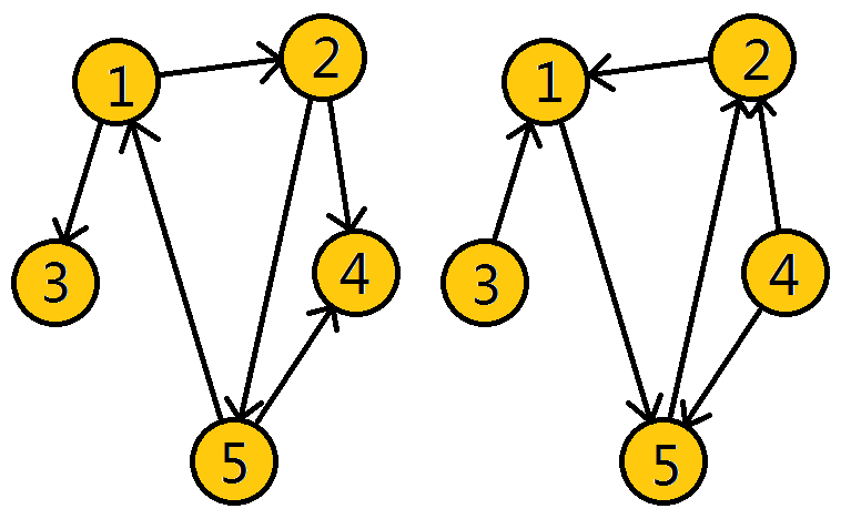
上图是有向图G , 和图G的逆图 GT
摘录维基百科上对Kosaraju Algorithm 的描述:
(取自https://en.wikipedia.org/wiki/Kosaraju%27s_algorithm)
- For each vertex u of the graph, mark u as unvisited. Let L be empty.
- For each vertex u of the graph do Visit(u), where Visit(u) is the recursive subroutine:
- If u is unvisited then:
- Mark u as visited.
- For each out-neighbour v of u, do Visit(v).
- Prepend u to L.
- Otherwise do nothing.
- If u is unvisited then:
- For each element u of L in order, do Assign(u,u) where Assign(u,root) is the recursive subroutine:
- If u has not been assigned to a component then:
- Assign u as belonging to the component whose root is root.
- For each in-neighbour v of u, do Assign(v,root).
- Otherwise do nothing.
- If u has not been assigned to a component then:
通过以上的描述我们发现,Kosaraju 算法就是分别对原图G 和它的逆图 GT 进行两遍DFS,即:
1).对原图G进行深度优先搜索,找出每个节点的完成时间(时间戳)
2).选择完成时间较大的节点开始,对逆图GT 搜索,能够到达的点构成一个强连通分量
3).如果所有节点未被遍历,重复2). ,否则算法结束;
二.算法图示

上图是对图G,进行一遍DFS的结果,每个节点有两个时间戳,即节点的发现时间u.d和完成时间u.f
我们将完成时间较大的,按大小加入堆栈
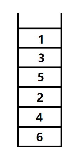
1)每次从栈顶取出元素
2)检查是否被访问过
3)若没被访问过,以该点为起点,对逆图进行深度优先遍历
4)否则返回第一步,直到栈空为止
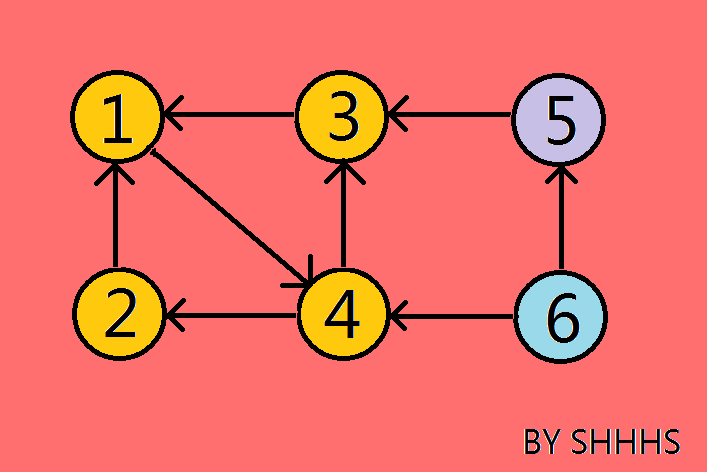
[ATTENTION] : 对逆图搜索时,从一个节点开始能搜索到的最大区块就是该点所在的强连通分量。
从节点1出发,能走到 2 ,3,4 , 所以{1 , 2 , 3 , 4 }是一个强连通分量
从节点5出发,无路可走,所以{ 5 }是一个强连通分量
从节点6出发,无路可走,所以{ 6 }是一个强连通分量
自此Kosaraju Algorithm完毕,这个算法只需要两遍DFS即可,是一个比较易懂的求强连通分量的算法。
STRONG-CONNECTED-COMPONENTS ( GRAPH G )
1 call DFS(G) to compute finishing times u.f for each vertex u
2 compute GT
3 call DFS (GT) , but in the main loop of DFS , consider the vertices
in order of decreasing u.f ( as computed in line 1 )
4 output the vertices of each tree in the depth-first forest formed in line 3 as a
separate strongly-connected-componet
三.算法复杂度
邻接表:O(V+E)
邻接矩阵:O(V2)
该算法在实际操作中要比Tarjan算法要慢
四.算法模板&注释代码
 1 #include "cstdio"
 2 #include "iostream"
 3 #include "algorithm"
 4
 5 using namespace std ;
 6
 7 const int maxN = 10010 , maxM = 50010;
 8
 9 struct Kosaraju { int to , next ; } ;
10
11 Kosaraju E[ 2 ][ maxM ] ;
12 bool vis[ maxN ];
13 int head[ 2 ][ maxN ] , cnt[ 2 ] , ord[maxN] , size[maxN] ,color[ maxN ];
14
15 int tot , dfs_num  , col_num , N , M  ;
16
17 void Add_Edge( int x , int y , int _ ){//建图
18          E[ _ ][ ++cnt[ _ ] ].to = y ;
19          E[ _ ][ cnt[ _ ] ].next = head[ _ ][ x ] ;
20          head[ _ ][ x ] = cnt[ _ ] ;
21 }
22
23 void DFS_1 ( int x , int _ ){
24          dfs_num ++ ;//发现时间
25          vis[ x ] = true ;
26          for ( int i = head[ _ ][ x ] ; i ; i = E[ _ ][ i ].next ) {
27                  int temp = E[ _ ][ i ].to;
28                  if(vis[ temp ] == false) DFS_1 ( temp , _ ) ;
29          }
30          ord[(N<<1) + 1 - (++dfs_num) ] = x ;//完成时间加入栈
31 }
32
33 void DFS_2 ( int x , int _ ){
34          size[ tot ]++ ;// 强连通分量的大小
35          vis[ x ] = false ;
36          color[ x ] = col_num ;//染色
37          for ( int i=head[ _ ][ x ] ; i ; i = E[ _ ][ i ].next ) {
38                  int temp = E[ _ ][ i ].to;
39                  if(vis[temp] == true) DFS_2(temp , _);
40          }
41 }
42
43 int main ( ){
44          scanf("%d %d" , &N , &M );
45          for ( int i=1 ; i<=M ; ++i ){
46                  int _x , _y ;
47                  scanf("%d %d" , &_x , &_y ) ;
48                  Add_Edge( _x , _y , 0 ) ;//原图的邻接表
49                  Add_Edge( _y , _x , 1 ) ;//逆图的邻接表
50          }
51          for ( int i=1 ; i<=N ; ++i )
52                  if ( vis[ i ]==false )
53                           DFS_1 ( i , 0 ) ;//原图的DFS
54
55          for ( int i = 1 ; i<=( N << 1) ; ++i ) {
56                  if( ord[ i ]!=0 && vis[ ord[ i ] ] ){
57                           tot ++ ; //强连通分量的个数
58                           col_num ++ ;//染色的颜色
59                           DFS_2 ( ord[ i ] , 1 ) ;
60                  }
61          }
62
63          for ( int i=1 ; i<=tot ; ++i )
64                  printf ("%d ",size[ i ]);
65          putchar ('
');
66          for ( int i=1 ; i<=N ; ++i )
67                  printf ("%d ",color[ i ]);
68          return 0;
69 }
2016-09-18 00:16:19
(完)