如何在pytorch中使用自定义的激活函数?
如果自定义的激活函数是可导的,那么可以直接写一个python function来定义并调用,因为pytorch的autograd会自动对其求导。
如果自定义的激活函数不是可导的,比如类似于ReLU的分段可导的函数,需要写一个继承torch.autograd.Function的类,并自行定义forward和backward的过程。
在pytorch中提供了定义新的autograd function的tutorial: https://pytorch.org/tutorials/beginner/examples_autograd/two_layer_net_custom_function.html, tutorial以ReLU为例介绍了在forward, backward中需要自行定义的内容。
 1 import torch
 2
 3
 4 class MyReLU(torch.autograd.Function):
 5     """
 6     We can implement our own custom autograd Functions by subclassing
 7     torch.autograd.Function and implementing the forward and backward passes
 8     which operate on Tensors.
 9     """
10
11     @staticmethod
12     def forward(ctx, input):
13         """
14         In the forward pass we receive a Tensor containing the input and return
15         a Tensor containing the output. ctx is a context object that can be used
16         to stash information for backward computation. You can cache arbitrary
17         objects for use in the backward pass using the ctx.save_for_backward method.
18         """
19         ctx.save_for_backward(input)
20         return input.clamp(min=0)
21
22     @staticmethod
23     def backward(ctx, grad_output):
24         """
25         In the backward pass we receive a Tensor containing the gradient of the loss
26         with respect to the output, and we need to compute the gradient of the loss
27         with respect to the input.
28         """
29         input, = ctx.saved_tensors
30         grad_input = grad_output.clone()
31         grad_input[input < 0] = 0
32         return grad_input
33
34
35 dtype = torch.float
36 device = torch.device("cpu")
37 # device = torch.device("cuda:0") # Uncomment this to run on GPU
38
39 # N is batch size; D_in is input dimension;
40 # H is hidden dimension; D_out is output dimension.
41 N, D_in, H, D_out = 64, 1000, 100, 10
42
43 # Create random Tensors to hold input and outputs.
44 x = torch.randn(N, D_in, device=device, dtype=dtype)
45 y = torch.randn(N, D_out, device=device, dtype=dtype)
46
47 # Create random Tensors for weights.
48 w1 = torch.randn(D_in, H, device=device, dtype=dtype, requires_grad=True)
49 w2 = torch.randn(H, D_out, device=device, dtype=dtype, requires_grad=True)
50
51 learning_rate = 1e-6
52 for t in range(500):
53     # To apply our Function, we use Function.apply method. We alias this as 'relu'.
54     relu = MyReLU.apply
55
56     # Forward pass: compute predicted y using operations; we compute
57     # ReLU using our custom autograd operation.
58     y_pred = relu(x.mm(w1)).mm(w2)
59
60     # Compute and print loss
61     loss = (y_pred - y).pow(2).sum()
62     print(t, loss.item())
63
64     # Use autograd to compute the backward pass.
65     loss.backward()
66
67     # Update weights using gradient descent
68     with torch.no_grad():
69         w1 -= learning_rate * w1.grad
70         w2 -= learning_rate * w2.grad
71
72         # Manually zero the gradients after updating weights
73         w1.grad.zero_()
74         w2.grad.zero_()
但是如果定义ReLU函数时,没有使用以上正确的方法,而是直接自定义的函数,会出现什么问题呢?
这里对比了使用以上MyReLU和自定义函数:no_back的实验结果。
1 def no_back(x):
2     return x * (x > 0).float()
代码:
N, D_in, H, D_out = 2, 3, 4, 5

# Create random Tensors to hold input and outputs.
x = torch.randn(N, D_in, device=device, dtype=dtype)
y = torch.randn(N, D_out, device=device, dtype=dtype)

# Create random Tensors for weights.
origin_w1 = torch.randn(D_in, H, device=device, dtype=dtype, requires_grad=True)
origin_w2 = torch.randn(H, D_out, device=device, dtype=dtype, requires_grad=True)

learning_rate = 1e-3

def myReLU(func, x, y, origin_w1, origin_w2, learning_rate,N = 2, D_in = 3, H = 4, D_out = 5):
    w1 = deepcopy(origin_w1)
    w2 = deepcopy(origin_w2)
    for t in range(5):
        # Forward pass: compute predicted y using operations; we compute
        # ReLU using our custom autograd operation.
        y_pred = func(x.mm(w1)).mm(w2)

        # Compute and print loss
        loss = (y_pred - y).pow(2).sum()
        print("------", t, loss.item(), "------------")

        # Use autograd to compute the backward pass.
        loss.backward()

        # Update weights using gradient descent
        with torch.no_grad():
            print('w1 = ')
            print(w1)
            print('---------------------')
            print("x.mm(w1) = ")
            print(x.mm(w1))
            print('---------------------')
            print('func(x.mm(w1))')
            print(func(x.mm(w1)))
            print('---------------------')
            print("w1.grad:", w1.grad)
            # print("w2.grad:",w2.grad)
            print('---------------------')

            w1 -= learning_rate * w1.grad
            w2 -= learning_rate * w2.grad

            # Manually zero the gradients after updating weights
            w1.grad.zero_()
            w2.grad.zero_()
            print('========================')
            print()


myReLU(func = MyReLU.apply, x = x, y = y, origin_w1 = origin_w1, origin_w2 = origin_w2, learning_rate = learning_rate, N = 2, D_in = 3, H = 4, D_out = 5)
print('============')
print('============')
print('============')
myReLU(func = no_back, x = x, y = y, origin_w1 = origin_w1, origin_w2 = origin_w2, learning_rate = learning_rate, N = 2, D_in = 3, H = 4, D_out = 5)
对于使用了MyReLU.apply的实验结果为:


 1 ------ 0 20.18220329284668 ------------
 2 w1 =
 3 tensor([[ 0.7070,  2.5772,  0.7987,  2.2287],
 4         [ 0.7425, -0.6309,  0.3268, -1.5072],
 5         [ 0.6930, -2.6128,  0.1949,  0.8819]], requires_grad=True)
 6 ---------------------
 7 x.mm(w1) =
 8 tensor([[-0.9788,  1.0135, -0.4164,  1.8834],
 9         [-0.7692, -1.8556, -0.7085, -0.9849]])
10 ---------------------
11 func(x.mm(w1))
12 tensor([[0.0000, 1.0135, 0.0000, 1.8834],
13         [0.0000, 0.0000, 0.0000, 0.0000]])
14 ---------------------
15 w1.grad: tensor([[  0.0000,   0.0499,   0.0000,   0.1881],
16         [  0.0000,  -4.4962,   0.0000, -16.9378],
17         [  0.0000,  -0.2401,   0.0000,  -0.9043]])
18 ---------------------
19 ========================
20
21 ------ 1 19.546737670898438 ------------
22 w1 =
23 tensor([[ 0.7070,  2.5772,  0.7987,  2.2285],
24         [ 0.7425, -0.6265,  0.3268, -1.4903],
25         [ 0.6930, -2.6126,  0.1949,  0.8828]], requires_grad=True)
26 ---------------------
27 x.mm(w1) =
28 tensor([[-0.9788,  1.0078, -0.4164,  1.8618],
29         [-0.7692, -1.8574, -0.7085, -0.9915]])
30 ---------------------
31 func(x.mm(w1))
32 tensor([[0.0000, 1.0078, 0.0000, 1.8618],
33         [0.0000, 0.0000, 0.0000, 0.0000]])
34 ---------------------
35 w1.grad: tensor([[  0.0000,   0.0483,   0.0000,   0.1827],
36         [  0.0000,  -4.3446,   0.0000, -16.4493],
37         [  0.0000,  -0.2320,   0.0000,  -0.8782]])
38 ---------------------
39 ========================
40
41 ------ 2 18.94647789001465 ------------
42 w1 =
43 tensor([[ 0.7070,  2.5771,  0.7987,  2.2283],
44         [ 0.7425, -0.6221,  0.3268, -1.4738],
45         [ 0.6930, -2.6123,  0.1949,  0.8837]], requires_grad=True)
46 ---------------------
47 x.mm(w1) =
48 tensor([[-0.9788,  1.0023, -0.4164,  1.8409],
49         [-0.7692, -1.8591, -0.7085, -0.9978]])
50 ---------------------
51 func(x.mm(w1))
52 tensor([[0.0000, 1.0023, 0.0000, 1.8409],
53         [0.0000, 0.0000, 0.0000, 0.0000]])
54 ---------------------
55 w1.grad: tensor([[  0.0000,   0.0467,   0.0000,   0.1775],
56         [  0.0000,  -4.2009,   0.0000, -15.9835],
57         [  0.0000,  -0.2243,   0.0000,  -0.8534]])
58 ---------------------
59 ========================
60
61 ------ 3 18.378826141357422 ------------
62 w1 =
63 tensor([[ 0.7070,  2.5771,  0.7987,  2.2281],
64         [ 0.7425, -0.6179,  0.3268, -1.4578],
65         [ 0.6930, -2.6121,  0.1949,  0.8846]], requires_grad=True)
66 ---------------------
67 x.mm(w1) =
68 tensor([[-0.9788,  0.9969, -0.4164,  1.8206],
69         [-0.7692, -1.8607, -0.7085, -1.0040]])
70 ---------------------
71 func(x.mm(w1))
72 tensor([[0.0000, 0.9969, 0.0000, 1.8206],
73         [0.0000, 0.0000, 0.0000, 0.0000]])
74 ---------------------
75 w1.grad: tensor([[  0.0000,   0.0451,   0.0000,   0.1726],
76         [  0.0000,  -4.0644,   0.0000, -15.5391],
77         [  0.0000,  -0.2170,   0.0000,  -0.8296]])
78 ---------------------
79 ========================
80
81 ------ 4 17.841421127319336 ------------
82 w1 =
83 tensor([[ 0.7070,  2.5770,  0.7987,  2.2280],
84         [ 0.7425, -0.6138,  0.3268, -1.4423],
85         [ 0.6930, -2.6119,  0.1949,  0.8854]], requires_grad=True)
86 ---------------------
87 x.mm(w1) =
88 tensor([[-0.9788,  0.9918, -0.4164,  1.8008],
89         [-0.7692, -1.8623, -0.7085, -1.0100]])
90 ---------------------
91 func(x.mm(w1))
92 tensor([[0.0000, 0.9918, 0.0000, 1.8008],
93         [0.0000, 0.0000, 0.0000, 0.0000]])
94 ---------------------
95 w1.grad: tensor([[  0.0000,   0.0437,   0.0000,   0.1679],
96         [  0.0000,  -3.9346,   0.0000, -15.1145],
97         [  0.0000,  -0.2101,   0.0000,  -0.8070]])
98 ---------------------
99 ========================
对于使用了no_back的实验结果为:
 1 ------ 0 20.18220329284668 ------------
 2 w1 =
 3 tensor([[ 0.7070,  2.5772,  0.7987,  2.2287],
 4         [ 0.7425, -0.6309,  0.3268, -1.5072],
 5         [ 0.6930, -2.6128,  0.1949,  0.8819]], requires_grad=True)
 6 ---------------------
 7 x.mm(w1) =
 8 tensor([[-0.9788,  1.0135, -0.4164,  1.8834],
 9         [-0.7692, -1.8556, -0.7085, -0.9849]])
10 ---------------------
11 func(x.mm(w1))
12 tensor([[-0.0000, 1.0135, -0.0000, 1.8834],
13         [-0.0000, -0.0000, -0.0000, -0.0000]])
14 ---------------------
15 w1.grad: tensor([[  0.0000,   0.0499,   0.0000,   0.1881],
16         [  0.0000,  -4.4962,   0.0000, -16.9378],
17         [  0.0000,  -0.2401,   0.0000,  -0.9043]])
18 ---------------------
19 ========================
20
21 ------ 1 19.546737670898438 ------------
22 w1 =
23 tensor([[ 0.7070,  2.5772,  0.7987,  2.2285],
24         [ 0.7425, -0.6265,  0.3268, -1.4903],
25         [ 0.6930, -2.6126,  0.1949,  0.8828]], requires_grad=True)
26 ---------------------
27 x.mm(w1) =
28 tensor([[-0.9788,  1.0078, -0.4164,  1.8618],
29         [-0.7692, -1.8574, -0.7085, -0.9915]])
30 ---------------------
31 func(x.mm(w1))
32 tensor([[-0.0000, 1.0078, -0.0000, 1.8618],
33         [-0.0000, -0.0000, -0.0000, -0.0000]])
34 ---------------------
35 w1.grad: tensor([[  0.0000,   0.0483,   0.0000,   0.1827],
36         [  0.0000,  -4.3446,   0.0000, -16.4493],
37         [  0.0000,  -0.2320,   0.0000,  -0.8782]])
38 ---------------------
39 ========================
40
41 ------ 2 18.94647789001465 ------------
42 w1 =
43 tensor([[ 0.7070,  2.5771,  0.7987,  2.2283],
44         [ 0.7425, -0.6221,  0.3268, -1.4738],
45         [ 0.6930, -2.6123,  0.1949,  0.8837]], requires_grad=True)
46 ---------------------
47 x.mm(w1) =
48 tensor([[-0.9788,  1.0023, -0.4164,  1.8409],
49         [-0.7692, -1.8591, -0.7085, -0.9978]])
50 ---------------------
51 func(x.mm(w1))
52 tensor([[-0.0000, 1.0023, -0.0000, 1.8409],
53         [-0.0000, -0.0000, -0.0000, -0.0000]])
54 ---------------------
55 w1.grad: tensor([[  0.0000,   0.0467,   0.0000,   0.1775],
56         [  0.0000,  -4.2009,   0.0000, -15.9835],
57         [  0.0000,  -0.2243,   0.0000,  -0.8534]])
58 ---------------------
59 ========================
60
61 ------ 3 18.378826141357422 ------------
62 w1 =
63 tensor([[ 0.7070,  2.5771,  0.7987,  2.2281],
64         [ 0.7425, -0.6179,  0.3268, -1.4578],
65         [ 0.6930, -2.6121,  0.1949,  0.8846]], requires_grad=True)
66 ---------------------
67 x.mm(w1) =
68 tensor([[-0.9788,  0.9969, -0.4164,  1.8206],
69         [-0.7692, -1.8607, -0.7085, -1.0040]])
70 ---------------------
71 func(x.mm(w1))
72 tensor([[-0.0000, 0.9969, -0.0000, 1.8206],
73         [-0.0000, -0.0000, -0.0000, -0.0000]])
74 ---------------------
75 w1.grad: tensor([[  0.0000,   0.0451,   0.0000,   0.1726],
76         [  0.0000,  -4.0644,   0.0000, -15.5391],
77         [  0.0000,  -0.2170,   0.0000,  -0.8296]])
78 ---------------------
79 ========================
80
81 ------ 4 17.841421127319336 ------------
82 w1 =
83 tensor([[ 0.7070,  2.5770,  0.7987,  2.2280],
84         [ 0.7425, -0.6138,  0.3268, -1.4423],
85         [ 0.6930, -2.6119,  0.1949,  0.8854]], requires_grad=True)
86 ---------------------
87 x.mm(w1) =
88 tensor([[-0.9788,  0.9918, -0.4164,  1.8008],
89         [-0.7692, -1.8623, -0.7085, -1.0100]])
90 ---------------------
91 func(x.mm(w1))
92 tensor([[-0.0000, 0.9918, -0.0000, 1.8008],
93         [-0.0000, -0.0000, -0.0000, -0.0000]])
94 ---------------------
95 w1.grad: tensor([[  0.0000,   0.0437,   0.0000,   0.1679],
96         [  0.0000,  -3.9346,   0.0000, -15.1145],
97         [  0.0000,  -0.2101,   0.0000,  -0.8070]])
98 ---------------------
99 ========================
对比发现,二者在梯度大小及更新的数值、loss大小等都是数值相等的,这是否说明对于不可导函数,直接定义函数也可以取得和正确定义前向后向过程相同的结果呢?
应当注意到一个问题,那就是在MyReLU.apply的实验结果中,出现数值为0的地方,显示为0.0000,而在no_back的实验结果中,出现数值为0的地方,显示为-0.0000;
0.0000与-0.0000有什么区别呢?
参考stack overflow中的解答:https://stackoverflow.com/questions/4083401/negative-zero-in-python
和wikipedia中对于signed zero的介绍:https://en.wikipedia.org/wiki/Signed_zero
在python中二者是显然不同的对象,但是在数值比较时,二者的值显示为相等。
-0.0 == +0.0 == 0
在Python 中使它们数值相等的设定,是在尽量避免为code引入bug.
>>> a = 3.4
>>> b =4.4
>>> c = -0.0
>>> d = +0.0
>>> a*c
-0.0
>>> b*d
0.0
>>> a*c == b*d
True
>>>
虽然看起来,它们在使用中并没有什么区别,但是在计算机内部对它们的编码表示并不相同。
在对于整数的1+7位元的符号数值表示法中,负零是用二进制代码10000000表示的。在8位元二进制反码中,负零是用二进制代码11111111表示,但补码表示法則沒有負零的概念。在IEEE 754二进制浮点数算术标准中,指数和尾数为零、符号位元为一的数就是负零。
在IBM的普通十进制算数编码规范中,运用十进制来表示浮点数。这里负零被表示为指数为编码内任意合法数值、所有系数均为零、符号位元为一的数。
~(wikipedia)
在数值分析中,也常将-0看做从负数区间无限趋近于0的值,将+0看做从正数区间无限趋近于0的值,二者在数值上近似相等,但在某些操作中却可能产生不同的结果。
比如 divmod,会沿用数值的sign:
>>> divmod(-0.0,100)
(-0.0, 0.0)
>>> divmod(+0.0,100)
(0.0, 0.0)
比如 atan2, (介绍详见https://en.wikipedia.org/wiki/Atan2)
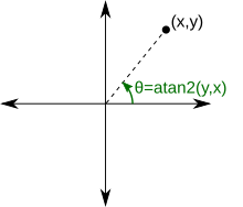
atan2(+0, +0) = +0;
atan2(+0, −0) = +π; ( 当y是位于y轴正半轴,无限趋近于0的值;x是位于x轴负半轴,无限趋近于0的值,=> 可以看做是在第二象限中位于x轴负半轴的一点 => $ heta夹角为$pi$)
atan2(−0, +0) = −0; ( 可以看做是在第四象限中位于x轴正半轴的一点 => $ heta夹角为-0)
atan2(−0, −0) = −π.
用代码验证:
>>> math.atan2(0.0, 0.0) == math.atan2(-0.0, 0.0)
True
>>> math.atan2(0.0, -0.0) == math.atan2(-0.0, -0.0)
False
所以,尽管在上面自定义激活函数时,将不可导函数强行加入到pytorch的autograd中运算,数值结果相同;但是注意到-0.0000的出现是程序有bug的提示,严谨考虑仍需要规范定义,如MyReLU。