Logistic Regression and Newton's Method

Data

For this exercise, suppose that a high school has a dataset representing 40 students who were admitted to college and 40 students who were not admitted. Each  training example contains a student's score on two standardized exams and a label of whether the student was admitted.

Your task is to build a binary classification model that estimates college admission chances based on a student's scores on two exams. In your training data,

a. The first column of your x array represents all Test 1 scores, and the second column represents all Test 2 scores.

b. The y vector uses '1' to label a student who was admitted and '0' to label a student who was not admitted.

Plot the data

Load the data for the training examples into your program and add the intercept term into your x matrix.

Before beginning Newton's Method, we will first plot the data using different symbols to represent the two classes. In Matlab/Octave, you can separate the positive class and the negative class using the find command:

% find returns the indices of the
% rows meeting the specified condition
pos = find(y == 1); neg = find(y == 0);

% Assume the features are in the 2nd and 3rd
% columns of x
plot(x(pos, 2), x(pos,3), '+'); hold on
plot(x(neg, 2), x(neg, 3), 'o')

Your plot should look like the following:

Newton's Method

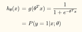
在logistic regression问题中，logistic函数表达式如下：

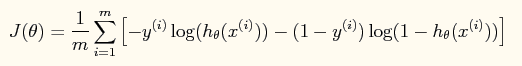
这样做的好处是可以把输出结果压缩到0~1之间。而在logistic回归问题中的损失函数与线性回归中的损失函数不同，这里定义的为：

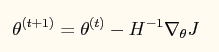
如果采用牛顿法来求解回归方程中的参数，则参数的迭代公式为：

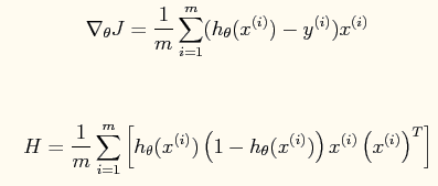
其中一阶导函数和hessian矩阵表达式如下：

code

% Exercise 4 -- Logistic Regression

clear all; close all; clc

x = load('ex4x.dat'); 
y = load('ex4y.dat');

[m, n] = size(x);

% Add intercept term to x
x = [ones(m, 1), x]; 

% Plot the training data
% Use different markers for positives and negatives
figure
pos = find(y); neg = find(y == 0);%find是找到的一个向量，其结果是find函数括号值为真时的值的编号
plot(x(pos, 2), x(pos,3), '+')
hold on
plot(x(neg, 2), x(neg, 3), 'o')
hold on
xlabel('Exam 1 score')
ylabel('Exam 2 score')


% Initialize fitting parameters
theta = zeros(n+1, 1);

% Define the sigmoid function 匿名函数
g = inline('1.0 ./ (1.0 + exp(-z))'); 

% Newton's method
MAX_ITR = 7;
J = zeros(MAX_ITR, 1);

for i = 1:MAX_ITR
    % Calculate the hypothesis function
    z = x * theta;
    h = g(z);%转换成logistic函数
    
    % Calculate gradient and hessian.
    % The formulas below are equivalent to the summation formulas
    % given in the lecture videos.
    grad = (1/m).*x' * (h-y);%梯度的矢量表示法
    H = (1/m).*x' * diag(h) * diag(1-h) * x;%hessian矩阵的矢量表示法
    
    % Calculate J (for testing convergence)
    J(i) =(1/m)*sum(-y.*log(h) - (1-y).*log(1-h));%损失函数的矢量表示法
    
    theta = theta - Hgrad;%是这样子的吗？
end
% Display theta
theta

% Calculate the probability that a student with
% Score 20 on exam 1 and score 80 on exam 2 
% will not be admitted
prob = 1 - g([1, 20, 80]*theta)

%画出分界面
% Plot Newton's method result
% Only need 2 points to define a line, so choose two endpoints
plot_x = [min(x(:,2))-2,  max(x(:,2))+2];
% Calculate the decision boundary line，plot_y的计算公式见博客下面的评论。
plot_y = (-1./theta(3)).*(theta(2).*plot_x +theta(1));
plot(plot_x, plot_y)
legend('Admitted', 'Not admitted', 'Decision Boundary')
hold off

% Plot J
figure
plot(0:MAX_ITR-1, J, 'o--', 'MarkerFaceColor', 'r', 'MarkerSize', 8)
xlabel('Iteration'); ylabel('J')
% Display J
J

matlab

diag函数功能：矩阵对角元素的提取和创建对角阵

设以下X为方阵，v为向量

1、X = diag(v,k)当v是一个含有n个元素的向量时，返回一个n+abs(k)阶方阵X，向量v在矩阵X中的第k个对角线上，k=0表示主对角线，k>0表示在主对角线上方，k<0表示在主对角线下方。例1：

v=[1 2 3];
diag(v, 3)

ans =

0  0  0  1  0  0
0  0  0  0  2  0
0  0  0  0  0  3
0  0  0  0  0  0
0  0  0  0  0  0
0  0  0  0  0  0

注：从主对角矩阵上方的第三个位置开始按对角线方向产生数据的

例2：

v=[1 2 3];
diag(v, -1)
ans =
0 0 0 0
1 0 0 0
0 2 0 0
0 0 3 0

注：从主对角矩阵下方的第一个位置开始按对角线方向产生数据的

2、X = diag(v)

向量v在方阵X的主对角线上，类似于diag(v,k),k=0的情况。

例3：

v=[1 2 3];
diag(v)

ans =

1 0 0
0 2 0
0 0 3

注：写成了对角矩阵的形式

3、v = diag(X,k)

返回列向量v，v由矩阵X的第k个对角线上的元素形成

例4：

v=[1 0 3;2 3 1;4 5 3];
diag(v,1)

ans =

0
1

注：把主对角线上方的第一个数据作为起始数据，按对角线顺序取出写成列向量形式

4、v = diag(X)返回矩阵X的主对角线上的元素，类似于diag(X,k)，k=0的情况例5：

v=[1 0 0;0 3 0;0 0 3];
diag(v)

ans =

1
3
3

或改为：

v=[1 0 3;2 3 1;4 5 3];
diag(v)

ans =

1
3
3

注：把主对角线的数据取出写成列向量形式

5、diag(diag(X))

取出X矩阵的对角元，然后构建一个以X对角元为对角的对角矩阵。
例6：

X=[1 2;3 4] 
diag(diag(X))

X =

1  2
3  4

ans =

1  0
0  4