前言:
这节主要是练习下PCA,PCA Whitening以及ZCA Whitening在2D数据上的使用,2D的数据集是45个数据点,每个数据点是2维的。参考的资料是:Exercise:PCA in 2D。结合前面的博文Deep learning:十(PCA和whitening)理论知识,来进一步理解PCA和Whitening的作用。
matlab某些函数:
scatter:
scatter(X,Y,<S>,<C>,’<type>’);
<S> – 点的大小控制,设为和X,Y同长度一维向量,则值决定点的大小;设为常数或缺省,则所有点大小统一。
<C> – 点的颜色控制,设为和X,Y同长度一维向量,则色彩由值大小线性分布;设为和X,Y同长度三维向量,则按colormap RGB值定义每点颜色,[0,0,0]是黑色,[1,1,1]是白色。缺省则颜色统一。
<type> – 点型:可选filled指代填充,缺省则画出的是空心圈。
plot:
plot可以用来画直线,比如说plot([1 2],[0 4])是画出一条连接(1,0)到(2,4)的直线,主要点坐标的对应关系。
实验过程:
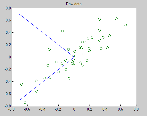
一、首先download这些二维数据,因为数据是以文本方式保存的,所以load的时候是以ascii码读入的。然后对输入样本进行协方差矩阵计算,并计算出该矩阵的SVD分解,得到其特征值向量,在原数据点上画出2条主方向,如下图所示:
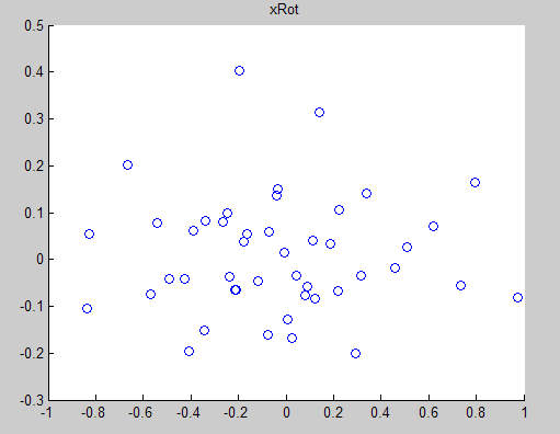
二、将经过PCA降维后的新数据在坐标中显示出来,如下图所示:
三、用新数据反过来重建原数据,其结果如下图所示:

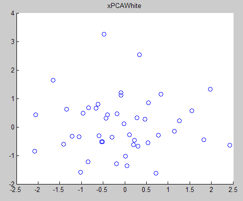
四、使用PCA whitening的方法得到原数据的分布情况如:
五、使用ZCA whitening的方法得到的原数据的分布如下所示:

PCA whitening和ZCA whitening不同之处在于处理后的结果数据的方差不同,尽管不同维度的方差是相等的。
实验代码:
close all

%%================================================================
%% Step 0: Load data
%  We have provided the code to load data from pcaData.txt into x.
%  x is a 2 * 45 matrix, where the kth column x(:,k) corresponds to
%  the kth data point.Here we provide the code to load natural image data into x.
%  You do not need to change the code below.

x = load('pcaData.txt','-ascii');
figure(1);
scatter(x(1, :), x(2, :));
title('Raw data');


%%================================================================
%% Step 1a: Implement PCA to obtain U
%  Implement PCA to obtain the rotation matrix U, which is the eigenbasis
%  sigma.

% -------------------- YOUR CODE HERE --------------------
u = zeros(size(x, 1)); % You need to compute this
[n m] = size(x);
%x = x-repmat(mean(x,2),1,m);%预处理,均值为0
sigma = (1.0/m)*x*x';
[u s v] = svd(sigma);


% --------------------------------------------------------
hold on
plot([0 u(1,1)], [0 u(2,1)]);%画第一条线
plot([0 u(1,2)], [0 u(2,2)]);%第二条线
scatter(x(1, :), x(2, :));
hold off

%%================================================================
%% Step 1b: Compute xRot, the projection on to the eigenbasis
%  Now, compute xRot by projecting the data on to the basis defined
%  by U. Visualize the points by performing a scatter plot.

% -------------------- YOUR CODE HERE --------------------
xRot = zeros(size(x)); % You need to compute this
xRot = u'*x;


% --------------------------------------------------------

% Visualise the covariance matrix. You should see a line across the
% diagonal against a blue background.
figure(2);
scatter(xRot(1, :), xRot(2, :));
title('xRot');

%%================================================================
%% Step 2: Reduce the number of dimensions from 2 to 1.
%  Compute xRot again (this time projecting to 1 dimension).
%  Then, compute xHat by projecting the xRot back onto the original axes
%  to see the effect of dimension reduction

% -------------------- YOUR CODE HERE --------------------
k = 1; % Use k = 1 and project the data onto the first eigenbasis
xHat = zeros(size(x)); % You need to compute this
xHat = u*([u(:,1),zeros(n,1)]'*x);


% --------------------------------------------------------
figure(3);
scatter(xHat(1, :), xHat(2, :));
title('xHat');


%%================================================================
%% Step 3: PCA Whitening
%  Complute xPCAWhite and plot the results.

epsilon = 1e-5;
% -------------------- YOUR CODE HERE --------------------
xPCAWhite = zeros(size(x)); % You need to compute this
xPCAWhite = diag(1./sqrt(diag(s)+epsilon))*u'*x;


% --------------------------------------------------------
figure(4);
scatter(xPCAWhite(1, :), xPCAWhite(2, :));
title('xPCAWhite');

%%================================================================
%% Step 3: ZCA Whitening
%  Complute xZCAWhite and plot the results.

% -------------------- YOUR CODE HERE --------------------
xZCAWhite = zeros(size(x)); % You need to compute this
xZCAWhite = u*diag(1./sqrt(diag(s)+epsilon))*u'*x;

% --------------------------------------------------------
figure(5);
scatter(xZCAWhite(1, :), xZCAWhite(2, :));
title('xZCAWhite');

%% Congratulations! When you have reached this point, you are done!
%  You can now move onto the next PCA exercise. :)
参考资料: