1.calcHist
计算一组数组的直方图。
- C++:
calcHist(const Mat* images, int nimages, const int* channels, InputArray mask, OutputArray hist, int dims, const int* histSize, const float** ranges, bool uniform=true, bool accumulate=false )
- C++:
calcHist(const Mat* images, int nimages, const int* channels, InputArray mask, SparseMat& hist, int dims, const int* histSize, const float** ranges, bool uniform=true, bool accumulate=false )
- C:
cvCalcHist(IplImage** image, CvHistogram* hist, int accumulate=0, const CvArr* mask=NULL )
-
Parameters: - images – 源数组。 它们都应具有相同的深度CV_8U或CV_32F和相同的大小。 它们每个都可以具有任意数量的通道。
- nimages – Number of source images.
- channels – 用于计算直方图的暗淡通道列表。 第一个数组通道的编号从0到images [0] .channels()-1,第二个数组通道的编号从images [0] .channels()到images [0] .channels()+ images [1]。 channel()-1,依此类推。
- mask – 可选的mask。 如果矩阵不为空,则它必须是大小与images [i]相同的8位数组。 非零掩码元素标记在直方图中计数的数组元素。
- hist –输出直方图,它是密集或稀疏的暗维数组。
- dims – 直方图维数必须为正且不大于CV_MAX_DIMS(在当前OpenCV版本中等于32)。
- histSize – 每个维度中的直方图大小数组
- ranges –每个维度中直方图bin边界的dims数组。 当直方图是均匀的(uniform = true)时,则对于每个维度i,足以指定第0个直方图bin的下(包含)边界L_0和上(专有)边界U _ { texttt {histSize} [ i] -1}表示最后一个直方图bin histSize [i] -1。 即,在均匀的直方图的情况下,range [i]中的每个都是2个元素的数组。 当直方图不均匀时(uniform = false),则每个range [i]都包含histSize [i] +1个元素:
![L_0, U_0=L_1, U_1=L_2, ..., U_{ exttt{histSize[i]}-2}=L_{ exttt{histSize[i]}-1}, U_{ exttt{histSize[i]}-1}](https://docs.opencv.org/2.4/_images/math/4aafe0a4c6ad01a75e608e213d5086c74ffae24a.png) . 不在
. 不在  and
and ![U_{ exttt{histSize[i]}-1}](https://docs.opencv.org/2.4/_images/math/bfd3f3bb827add85c2b87f8dee58dad2e396542e.png) 之内的元素, 不计入直方图内。
之内的元素, 不计入直方图内。 - uniform – 指示直方图是否均匀的标志。
- accumulate – 累积标志。 如果已设置,则分配直方图时不会在开始时清除它。 此功能使您可以从几组数组中计算单个直方图,或者及时更新直方图。
函数calcHist计算一个或多个数组的直方图。 用于增加直方图bin的元组的元素取自同一位置的相应输入数组。 下面的示例显示了如何为彩色图像计算2D色相饱和度直方图。
#include <cv.h>
#include <highgui.h>

using namespace cv;

int main( int argc, char** argv )
{
    Mat src, hsv;
    if( argc != 2 || !(src=imread(argv[1], 1)).data )
        return -1;

    cvtColor(src, hsv, CV_BGR2HSV);

    // Quantize the hue to 30 levels
    // and the saturation to 32 levels
    int hbins = 30, sbins = 32;
    int histSize[] = {hbins, sbins};
    // hue varies from 0 to 179, see cvtColor
    float hranges[] = { 0, 180 };
    // saturation varies from 0 (black-gray-white) to
    // 255 (pure spectrum color)
    float sranges[] = { 0, 256 };
    const float* ranges[] = { hranges, sranges };
    MatND hist;
    // we compute the histogram from the 0-th and 1-st channels
    int channels[] = {0, 1};

    calcHist( &hsv, 1, channels, Mat(), // do not use mask
             hist, 2, histSize, ranges,
             true, // the histogram is uniform
             false );
    double maxVal=0;
    minMaxLoc(hist, 0, &maxVal, 0, 0);

    int scale = 10;
    Mat histImg = Mat::zeros(sbins*scale, hbins*10, CV_8UC3);

    for( int h = 0; h < hbins; h++ )
        for( int s = 0; s < sbins; s++ )
        {
            float binVal = hist.at<float>(h, s);
            int intensity = cvRound(binVal*255/maxVal);
            rectangle( histImg, Point(h*scale, s*scale),
                        Point( (h+1)*scale - 1, (s+1)*scale - 1),
                        Scalar::all(intensity),
                        CV_FILLED );
        }

    namedWindow( "Source", 1 );
    imshow( "Source", src );

    namedWindow( "H-S Histogram", 1 );
    imshow( "H-S Histogram", histImg );
    waitKey();
}
Note- An example for creating histograms of an image can be found at opencv_source_code/samples/cpp/demhist.cpp
2.calcBackProject
- C++:
calcBackProject(const Mat* images, int nimages, const int* channels, InputArray hist, OutputArray backProject, const float** ranges, double scale=1, bool uniform=true )
- C++:
calcBackProject(const Mat* images, int nimages, const int* channels, const SparseMat& hist, OutputArray backProject, const float** ranges, double scale=1, bool uniform=true )
- C:
cvCalcBackProject(IplImage** image, CvArr* backProject, const CvHistogram* hist)
-
Parameters: - images – Source arrays. They all should have the same depth,
CV_8UorCV_32F, and the same size. Each of them can have an arbitrary number of channels. - nimages – Number of source images.
- channels – The list of channels used to compute the back projection. The number of channels must match the histogram dimensionality. The first array channels are numerated from 0 to
images[0].channels()-1, the second array channels are counted fromimages[0].channels()toimages[0].channels() + images[1].channels()-1, and so on. - hist – Input histogram that can be dense or sparse.
- backProject – Destination back projection array that is a single-channel array of the same size and depth as
images[0]. - ranges – Array of arrays of the histogram bin boundaries in each dimension. See
calcHist(). - scale – Optional scale factor for the output back projection.
- uniform – Flag indicating whether the histogram is uniform or not (see above).
- images – Source arrays. They all should have the same depth,
函数calcBackProject计算直方图的后向项目。也就是说,类似于calcHist,该函数在每个位置(x,y)收集输入图像中所选通道的值,并找到对应的直方图bin。但是该函数不是增加它,而是读取bin值,按比例缩放它的值,然后存储在backProject(x,y)中。在统计方面,该函数根据直方图表示的经验概率分布计算每个元素值的概率。例如,查看如何在场景中查找和跟踪色彩鲜艳的对象:
跟踪之前,请向相机展示物体,以使其几乎覆盖整个画面。计算色调直方图。直方图可能具有很强的最大值,对应于对象中的主要颜色。
跟踪时,请使用该预先计算的直方图计算每个输入视频帧的色相平面的反投影。限制背投阈值以抑制较弱的色彩。抑制色彩饱和度不足且像素太暗或太亮的像素也可能是有意义的。
在结果图片中找到连接的组件,然后选择最大的组件。
This is an approximate algorithm of the CamShift() color object tracker.
See also
calcHist()3.compareHist
比较两个直方图。
- C++:
compareHist(InputArray H1, InputArray H2, int method)
- C++:
compareHist(const SparseMat& H1, const SparseMat& H2, int method)
- C:
cvCompareHist(const CvHistogram* hist1, const CvHistogram* hist2, int method)
-
Parameters: - H1 – First compared histogram.
- H2 – Second compared histogram of the same size as
H1. - method –
Comparison method that could be one of the following:
- CV_COMP_CORREL Correlation
- CV_COMP_CHISQR Chi-Square
- CV_COMP_INTERSECT Intersection
- CV_COMP_BHATTACHARYYA Bhattacharyya distance
- CV_COMP_HELLINGER Synonym for
CV_COMP_BHATTACHARYYA
compareHist函数使用指定的方法比较两个密集或两个稀疏直方图:
-
Correlation (
method=CV_COMP_CORREL)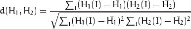
where
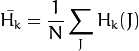
and
 is a total number of histogram bins.
 -
Chi-Square (
method=CV_COMP_CHISQR)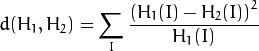
-
Intersection (
method=CV_COMP_INTERSECT)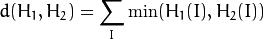
-
Bhattacharyya distance (
method=CV_COMP_BHATTACHARYYAormethod=CV_COMP_HELLINGER). In fact, OpenCV computes Hellinger distance, which is related to Bhattacharyya coefficient.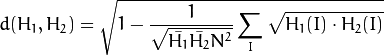
The function returns  .
.
虽然此功能可以很好地处理1、2、3维密集直方图,但它可能不适用于高维稀疏直方图。 在这种直方图中,由于混叠和采样问题,非零直方图块的坐标可能会略有偏移。 若要比较此类直方图或加权点的更一般的稀疏配置,请考虑使用EMD()函数。
4.EMD
计算两个加权点配置之间的“最小功”距离。
- C++:
EMD(InputArray signature1, InputArray signature2, int distType, InputArray cost=noArray(), float* lowerBound=0, OutputArray flow=noArray() )
- C:
cvCalcEMD2(const CvArr* signature1, const CvArr* signature2, int distance_type, CvDistanceFunction distance_func=NULL, const CvArr* cost_matrix=NULL, CvArr* flow=NULL, float* lower_bound=NULL, void* userdata=NULL )
-
Parameters: - signature1 – First signature, a
 floating-point matrix. Each row stores the point weight followed by the point coordinates. The matrix is allowed to have a single column (weights only) if the user-defined cost matrix is used.
 - signature2 – Second signature of the same format as
signature1, though the number of rows may be different. The total weights may be different. In this case an extra “dummy” point is added to eithersignature1orsignature2. - distType – Used metric.
CV_DIST_L1, CV_DIST_L2, andCV_DIST_Cstand for one of the standard metrics.CV_DIST_USERmeans that a pre-calculated cost matrixcostis used. - distance_func –
Custom distance function supported by the old interface.
CvDistanceFunctionis defined as:typedef float (CV_CDECL * CvDistanceFunction)( const float* a, const float* b, void* userdata );where
aandbare point coordinates anduserdatais the same as the last parameter. - cost – User-defined
 cost matrix. Also, if a cost matrix is used, lower boundary
 lowerBoundcannot be calculated because it needs a metric function. - lowerBound – Optional input/output parameter: lower boundary of a distance between the two signatures that is a distance between mass centers. The lower boundary may not be calculated if the user-defined cost matrix is used, the total weights of point configurations are not equal, or if the signatures consist of weights only (the signature matrices have a single column). You mustinitialize
*lowerBound. If the calculated distance between mass centers is greater or equal to*lowerBound(it means that the signatures are far enough), the function does not calculate EMD. In any case*lowerBoundis set to the calculated distance between mass centers on return. Thus, if you want to calculate both distance between mass centers and EMD,*lowerBoundshould be set to 0. - flow – Resultant
 flow matrix:
  is a flow from
  -th point of
 signature1to -th point of
 signature2. - userdata – Optional pointer directly passed to the custom distance function.
- signature1 – First signature, a
该函数计算推土机距离和/或两个加权点配置之间的距离的下边界。 [RubnerSept98]中描述的应用之一是用于图像检索的多维直方图比较。 EMD是使用单形算法的某些修改解决的运输问题,因此,在最坏的情况下,复杂度是指数级的,但是平均而言,它要快得多。 在实数的情况下,下边界可以更快地计算(使用线性时间算法),并且可以用来大致确定两个签名是否足够远,以致它们不能与同一对象相关。
5.equalizeHist
- C++:
equalizeHist(InputArray src, OutputArray dst)
- C:
cvEqualizeHist(const CvArr* src, CvArr* dst) -
Parameters: - src – Source 8-bit single channel image.
- dst – Destination image of the same size and type as
src.
-
Calculate the histogram
 for
for src. -
Normalize the histogram so that the sum of histogram bins is 255.
-
Compute the integral of the histogram:

-
Transform the image using
 as a look-up table:
6.Extra Histogram Functions (C API)
本节的其余部分描述了在CvHistogram上运行的其他C函数。
7.CalcBackProjectPatch
- C:
cvCalcBackProjectPatch(IplImage** images, CvArr* dst, CvSize patch_size, CvHistogram* hist, int method, double factor)
-
Parameters: - images – Source images (though, you may pass CvMat** as well).
- dst – Destination image.
- patch_size – Size of the patch slid though the source image.
- hist – Histogram.
- method – Comparison method passed to
CompareHist()(see the function description). - factor – Normalization factor for histograms that affects the normalization scale of the destination image. Pass 1 if not sure.
该功能通过将源图像块的直方图与给定的直方图进行比较来计算反投影。 该函数与matchTemplate()类似,但是函数CalcBackProjectPatch比较直方图,而不是将栅格面片与其在搜索窗口内的所有可能位置进行比较。 请参见下面的算法图:

8.CalcProbDensity
- C:
cvCalcProbDensity(const CvHistogram* hist1, const CvHistogram* hist2, CvHistogram* dst_hist, double scale=255 )
-
Parameters: - hist1 – First histogram (the divisor).
- hist2 – Second histogram.
- dst_hist – Destination histogram.
- scale – Scale factor for the destination histogram.

9.ClearHist
- C:
cvClearHist(CvHistogram* hist)
-
Parameters: hist – Histogram.
The function sets all of the histogram bins to 0 in case of a dense histogram and removes all histogram bins in case of a sparse array.
10.CopyHist
复制直方图。
- C:
cvCopyHist(const CvHistogram* src, CvHistogram** dst) -
Parameters: - src – Source histogram.
- dst – Pointer to the destination histogram.
该函数复制直方图。 如果第二个直方图指针* dst为NULL,则创建一个与src大小相同的新直方图。 否则,两个直方图必须具有相同的类型和大小。 然后,该函数将源直方图的bin值复制到目标直方图,并设置与src中相同的bin值范围。
11.CreateHist
创建直方图。
- C:
cvCreateHist(int dims, int* sizes, int type, float** ranges=NULL, int uniform=1 )
- Python:
cv.CreateHist(dims, type, ranges=None, uniform=1) → hist -
Parameters: - dims – Number of histogram dimensions.
- sizes – Array of the histogram dimension sizes.
- type – Histogram representation format.
CV_HIST_ARRAYmeans that the histogram data is represented as a multi-dimensional dense array CvMatND.CV_HIST_SPARSEmeans that histogram data is represented as a multi-dimensional sparse arrayCvSparseMat. - ranges – Array of ranges for the histogram bins. Its meaning depends on the
uniformparameter value. The ranges are used when the histogram is calculated or backprojected to determine which histogram bin corresponds to which value/tuple of values from the input image(s). - uniform – Uniformity flag. If not zero, the histogram has evenly spaced bins and for every
ranges[i]is an array of two numbers: lower and upper boundaries for the i-th histogram dimension. The whole range [lower,upper] is then split intodims[i]equal parts to determine thei-th input tuple value ranges for every histogram bin. And ifuniform=0, then thei-th element of therangesarray containsdims[i]+1elements:![exttt{lower}_0, exttt{upper}_0,
exttt{lower}_1, exttt{upper}_1 = exttt{lower}_2,
...
exttt{upper}_{dims[i]-1}](https://docs.opencv.org/2.4/_images/math/2c7b6f71211ef798aee15c7346320ca3560b0ee5.png) where
where  and
and  are lower and upper boundaries of the
 i-th input tuple value for thej-th bin, respectively. In either case, the input values that are beyond the specified range for a histogram bin are not counted byCalcHist()and filled with 0 byCalcBackProject().
该函数创建指定大小的直方图,并返回指向创建的直方图的指针。 如果数组范围是0,则必须稍后通过函数SetHistBinRanges()指定直方图bin范围。 尽管CalcHist()和CalcBackProject()可以在不设置bin范围的情况下处理8位图像,但它们假定它们在0到255个bin中等间隔。
12.GetMinMaxHistValue
- C:
cvGetMinMaxHistValue(const CvHistogram* hist, float* min_value, float* max_value, int* min_idx=NULL, int* max_idx=NULL )
- Python:
cv.GetMinMaxHistValue(hist)-> (min_value, max_value, min_idx, max_idx) -
Parameters: - hist – Histogram.
- min_value – Pointer to the minimum value of the histogram.
- max_value – Pointer to the maximum value of the histogram.
- min_idx – Pointer to the array of coordinates for the minimum.
- max_idx – Pointer to the array of coordinates for the maximum.
该函数查找最小和最大直方图块及其位置。 所有输出参数都是可选的。 在具有相同值的几个极值中,返回具有最小索引(按词典顺序)的极值。 如果有几个最大值或最小值,则以字典顺序(极值位置)中最早的形式返回。
13.MakeHistHeaderForArray
- C:
cvMakeHistHeaderForArray(int dims, int* sizes, CvHistogram* hist, float* data, float** ranges=NULL, int uniform=1 ) -
Parameters: - dims – Number of the histogram dimensions.
- sizes – Array of the histogram dimension sizes.
- hist – Histogram header initialized by the function.
- data – Array used to store histogram bins.
- ranges – Histogram bin ranges. See
CreateHist()for details. - uniform – Uniformity flag. See
CreateHist()for details.
该函数初始化直方图,其标题和箱由用户分配。 之后不需要调用ReleaseHist()。 这样只能初始化密集的直方图。 该函数返回hist。
14.NormalizeHist
- C:
cvNormalizeHist(CvHistogram* hist, double factor)
-
Parameters: - hist – Pointer to the histogram.
- factor – Normalization factor.
15.ReleaseHist
释放掉直方图。
- C:
cvReleaseHist(CvHistogram** hist) -
Parameters: - hist – Double pointer to the released histogram.
16.SetHistBinRanges
- C:
cvSetHistBinRanges(CvHistogram* hist, float** ranges, int uniform=1 ) -
Parameters: - hist – Histogram.
- ranges – Array of bin ranges arrays. See
CreateHist()for details. - uniform – Uniformity flag. See
CreateHist()for details.
17.ThreshHist
- C:
cvThreshHist(CvHistogram* hist, double threshold)
-
Parameters: - hist – Pointer to the histogram.
- threshold – Threshold level.