参考:https://blog.csdn.net/u013733326/article/details/79702148
希望大家直接到上面的网址去查看代码,下面是本人的笔记
建立一个带有隐藏层的神经网络
导入一些软件包
numpy:是用Python进行科学计算的基本软件包。
sklearn:为数据挖掘和数据分析提供的简单高效的工具。
matplotlib :是一个用于在Python中绘制图表的库。
testCases:提供了一些测试示例来评估函数的正确性,参见下载的资料或者在底部查看它的代码。
planar_utils :提供了在这个任务中使用的各种有用的功能,参见下载的资料或者在底部查看它的代码。
1.导入数据:
numpy.linspace(start, stop[, num=50[, endpoint=True[, retstep=False[, dtype=None]]]]])
返回在指定范围内的均匀间隔的数字(组成的数组),也即返回一个等差数列,参数说明:
- start - 起始点
- stop - 结束点
- num - 元素个数,默认为50,
- endpoint - 是否包含stop数值,默认为True,包含stop值;若为False,则不包含stop值
- retstep - 返回值形式,默认为False,返回等差数列组,若为True,则返回结果(array([`samples`]),`step`),
- dtype - 返回结果的数据类型,默认无,若无,则参考输入数据类型。
举例说明:
c = np.linspace(1,15,5,endpoint= False,retstep = False)
print(c) #[ 1.   3.8  6.6  9.4 12.2]
d = np.linspace(1,15,5,retstep = True)
print(d) #(array([ 1. ,  4.5,  8. , 11.5, 15. ]), 3.5)
代码:
import numpy as np
import matplotlib.pyplot as plt
import sklearn
import sklearn.datasets
import sklearn.linear_model

#要使用的数据集, 下面的代码会将一个花的图案的2类数据集加载到变量X和Y中。
def load_planar_dataset():
    np.random.seed(1)
    m = 400 # number of examples
    N = int(m/2) # number of points per class
    D = 2 # dimensionality
    X = np.zeros((m,D)) # m=400个点,每个点使用(x,y)表示,所以D=2,因此生成一个400*2的数据矩阵
    Y = np.zeros((m,1), dtype='uint8') # 标签向量,表明每个点的类型,0为红色,1位蓝色
    a = 4 # maximum ray of the flower

    for j in range(2):
        ix = range(N*j,N*(j+1)) #(0,200)和(200,400)
        t = np.linspace(j*3.12,(j+1)*3.12,N) + np.random.randn(N)*0.2 # theta
        r = a*np.sin(4*t) + np.random.randn(N)*0.2 # radius
        X[ix] = np.c_[r*np.sin(t), r*np.cos(t)]
        Y[ix] = j

    X = X.T
    Y = Y.T

    return X, Y
X, Y = load_planar_dataset()

plt.scatter(X[0, :], X[1, :], c=np.squeeze(Y), s=40, cmap=plt.cm.Spectral)#绘制散点图
返回:
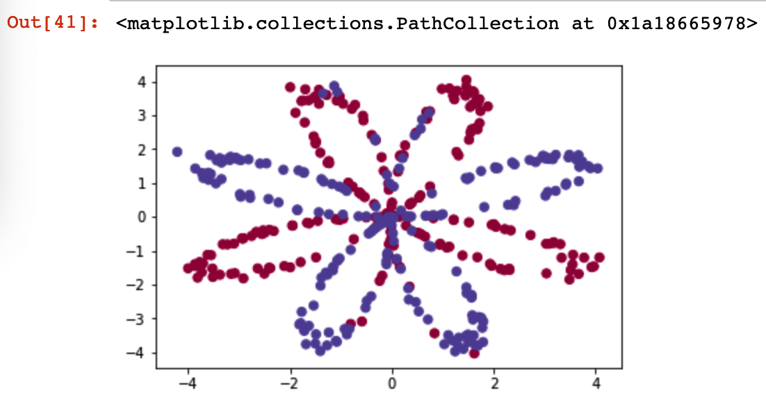
该神经网络的目标是建立一个模型来适应这些数据,将蓝色的点和红色的点分隔开来
- X:一个numpy的矩阵,包含了这些数据点的数值
- Y:一个numpy的向量,对应着的是X的标签【0 | 1】(红色:0 , 蓝色 :1)
2.如果试着使用logistic回归来进行分类
在构建完整的神经网络之前,先让我们看看逻辑回归在这个问题上的表现如何,我们可以使用sklearn的内置函数来做到这一点, 运行下面的代码来训练数据集上的逻辑回归分类器。
clf = sklearn.linear_model.LogisticRegressionCV()
clf.fit(X.T,Y.T)
会有警告:
/anaconda3/lib/python3.7/site-packages/sklearn/utils/validation.py:761: DataConversionWarning: A column-vector y was passed when a 1d array was expected. Please change the shape of y to (n_samples, ), for example using ravel().
  y = column_or_1d(y, warn=True)
/anaconda3/lib/python3.7/site-packages/sklearn/model_selection/_split.py:2053: FutureWarning: You should specify a value for 'cv' instead of relying on the default value. The default value will change from 3 to 5 in version 0.22.
  warnings.warn(CV_WARNING, FutureWarning)
返回:
LogisticRegressionCV(Cs=10, class_weight=None, cv='warn', dual=False,
           fit_intercept=True, intercept_scaling=1.0, max_iter=100,
           multi_class='warn', n_jobs=None, penalty='l2',
           random_state=None, refit=True, scoring=None, solver='lbfgs',
           tol=0.0001, verbose=0)
然后把逻辑回归分类器的分类绘制出来:
def plot_decision_boundary(model, X, y):
    #用于绘制logistic的线形分类线
    # Set min and max values and give it some padding
    x_min, x_max = X[0, :].min() - 1, X[0, :].max() + 1
    y_min, y_max = X[1, :].min() - 1, X[1, :].max() + 1
    h = 0.01
    # Generate a grid of points with distance h between them
    xx, yy = np.meshgrid(np.arange(x_min, x_max, h), np.arange(y_min, y_max, h))
    # Predict the function value for the whole grid
    Z = model(np.c_[xx.ravel(), yy.ravel()])
    Z = Z.reshape(xx.shape)
    # Plot the contour and training examples
    plt.contourf(xx, yy, Z, cmap=plt.cm.Spectral)
    plt.ylabel('x2')
    plt.xlabel('x1')
    plt.scatter(X[0, :], X[1, :], c=np.squeeze(y), cmap=plt.cm.Spectral)

plot_decision_boundary(lambda x: clf.predict(x), X, Y) #绘制决策边界
plt.title("Logistic Regression") #图标题
LR_predictions  = clf.predict(X.T) #预测结果
print ("逻辑回归的准确性: %d " % float((np.dot(Y, LR_predictions) +
        np.dot(1 - Y,1 - LR_predictions)) / float(Y.size) * 100) +
       "% " + "(正确标记的数据点所占的百分比)")
返回:
逻辑回归的准确性: 47 % (正确标记的数据点所占的百分比)
图示为:
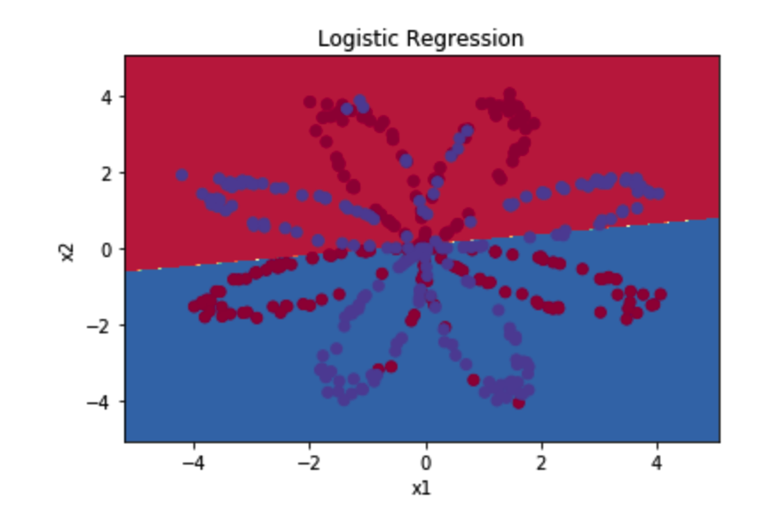
准确性只有47%的原因是数据集不是线性可分的,所以逻辑回归表现不佳,现在我们正式开始构建带有一层隐藏层的神经网络。
3.定义神经网络结构
隐藏层的神经元设置为4
def layer_sizes(X , Y):
    """
    参数:
     X - 输入数据集,维度为(输入的数量,训练/测试的数量)
     Y - 标签,维度为(输出的数量,训练/测试数量)

    返回:
     n_x - 输入层的数量
     n_h - 隐藏层的数量
     n_y - 输出层的数量
    """
    n_x = X.shape[0] #输入层
    n_h = 4 #,隐藏层,硬编码为4
    n_y = Y.shape[0] #输出层

    return (n_x,n_h,n_y)

#测试layer_sizes
print("=========================测试layer_sizes=========================")

def layer_sizes_test_case():
    np.random.seed(1)
    X_assess = np.random.randn(5, 3) #5个输入,训练/测试的数量为3
    Y_assess = np.random.randn(2, 3) #2个输出,训练/测试的数量为3
    return X_assess, Y_assess

X_asses , Y_asses = layer_sizes_test_case()
(n_x,n_h,n_y) =  layer_sizes(X_asses,Y_asses)
print("输入层的节点数量为: n_x = " + str(n_x))
print("隐藏层的节点数量为: n_h = " + str(n_h))
print("输出层的节点数量为: n_y = " + str(n_y))
返回:
=========================测试layer_sizes=========================
输入层的节点数量为: n_x = 5
隐藏层的节点数量为: n_h = 4
输出层的节点数量为: n_y = 2
4.初始化模型参数
进行随机初始化权重矩阵:
np.random.randn(a,b)* 0.01来随机初始化一个维度为(a,b)的矩阵。
将b初始化为零
np.random.seed(2)的作用是用于保证你得到的随机参数和作者的一样
def initialize_parameters( n_x , n_h ,n_y):
    """
    参数:
        n_x - 输入层节点的数量
        n_h - 隐藏层节点的数量
        n_y - 输出层节点的数量

    返回:
        parameters - 包含参数的字典:
            W1 - 权重矩阵,维度为(n_h,n_x)
            b1 - 偏向量,维度为(n_h,1)
            W2 - 权重矩阵,维度为(n_y,n_h)
            b2 - 偏向量,维度为(n_y,1)

    """
    np.random.seed(2) #指定一个随机种子,以便你的输出与我们的一样。
    W1 = np.random.randn(n_h,n_x) * 0.01
    b1 = np.zeros(shape=(n_h, 1))
    W2 = np.random.randn(n_y,n_h) * 0.01
    b2 = np.zeros(shape=(n_y, 1))

    #使用断言确保我的数据格式是正确的
    assert(W1.shape == ( n_h , n_x ))
    assert(b1.shape == ( n_h , 1 ))
    assert(W2.shape == ( n_y , n_h ))
    assert(b2.shape == ( n_y , 1 ))

    parameters = {"W1" : W1,
                  "b1" : b1,
                  "W2" : W2,
                  "b2" : b2 }

    return parameters

#测试initialize_parameters
print("=========================测试initialize_parameters=========================")

def initialize_parameters_test_case():
    n_x, n_h, n_y = 2, 4, 1
    return n_x, n_h, n_y

n_x , n_h , n_y = initialize_parameters_test_case()
parameters = initialize_parameters(n_x , n_h , n_y)
print("W1 = " + str(parameters["W1"]))
print("b1 = " + str(parameters["b1"]))
print("W2 = " + str(parameters["W2"]))
print("b2 = " + str(parameters["b2"]))
返回:
=========================测试initialize_parameters=========================
W1 = [[-0.00416758 -0.00056267]
 [-0.02136196  0.01640271]
 [-0.01793436 -0.00841747]
 [ 0.00502881 -0.01245288]]
b1 = [[0.]
 [0.]
 [0.]
 [0.]]
W2 = [[-0.01057952 -0.00909008  0.00551454  0.02292208]]
b2 = [[0.]]
5.前向传播
步骤如下:
- 使用字典类型的parameters(它是initialize_parameters() 的输出)检索每个参数。
- 实现向前传播, 计算Z[1],A[1],Z[2]和 A[2](训练集里面所有例子的预测向量)。
- 反向传播所需的值存储在“cache”中,cache将作为反向传播函数的输入。
隐藏层使用np.tanh()函数,输出层使用sigmoid()函数用于二分类,得到是红点还是蓝点
np.random.seed(1)的作用是用于保证后面操作中随机生成的X,Y都相等
def forward_propagation( X , parameters ):
    """
    参数:
         X - 维度为(n_x,m)的输入数据。
         parameters - 初始化函数(initialize_parameters)的输出

    返回:
         A2 - 使用sigmoid()函数计算的第二次激活后的数值
         cache - 包含“Z1”,“A1”,“Z2”和“A2”的字典类型变量
     """
    W1 = parameters["W1"]
    b1 = parameters["b1"]
    W2 = parameters["W2"]
    b2 = parameters["b2"]
    #前向传播计算A2
    Z1 = np.dot(W1 , X) + b1
    A1 = np.tanh(Z1)
    Z2 = np.dot(W2 , A1) + b2
    A2 = sigmoid(Z2)
    #使用断言确保我的数据格式是正确的
    assert(A2.shape == (1,X.shape[1]))
    cache = {"Z1": Z1,
             "A1": A1,
             "Z2": Z2,
             "A2": A2}

    return (A2, cache)

#测试forward_propagation
print("=========================测试forward_propagation=========================")

def forward_propagation_test_case():
    np.random.seed(1)
    X_assess = np.random.randn(2, 3) #两个输入,训练/测试数据有3个

    parameters = {'W1': np.array([[-0.00416758, -0.00056267], #将之前测试初始化参数时得到的值作为参数
        [-0.02136196,  0.01640271],
        [-0.01793436, -0.00841747],
        [ 0.00502881, -0.01245288]]),
     'W2': np.array([[-0.01057952, -0.00909008,  0.00551454,  0.02292208]]),
     'b1': np.array([[ 0.],
        [ 0.],
        [ 0.],
        [ 0.]]),
     'b2': np.array([[ 0.]])}

    return X_assess, parameters
X_assess, parameters = forward_propagation_test_case()
A2, cache = forward_propagation(X_assess, parameters)
print(A2)
print(cache)
print(np.mean(cache["Z1"]), np.mean(cache["A1"]), np.mean(cache["Z2"]), np.mean(cache["A2"]))
返回:
=========================测试forward_propagation=========================
[[0.5002307  0.49985831 0.50023963]]
{'Z1': array([[-0.00616586,  0.0020626 ,  0.0034962 ],
       [-0.05229879,  0.02726335, -0.02646869],
       [-0.02009991,  0.00368692,  0.02884556],
       [ 0.02153007, -0.01385322,  0.02600471]]), 'A1': array([[-0.00616578,  0.0020626 ,  0.00349619],
       [-0.05225116,  0.02725659, -0.02646251],
       [-0.02009721,  0.0036869 ,  0.02883756],
       [ 0.02152675, -0.01385234,  0.02599885]]), 'Z2': array([[ 0.00092281, -0.00056678,  0.00095853]]), 'A2': array([[0.5002307 , 0.49985831, 0.50023963]])}
-0.0004997557777419902 -0.000496963353231779 0.00043818745095914653 0.500109546852431
6.计算成本
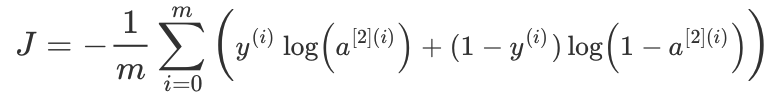
def compute_cost(A2,Y):
    """
    计算方程(6)中给出的交叉熵成本,

    参数:
         A2 - 使用sigmoid()函数计算的第二次激活后的数值
         Y - "True"标签向量,维度为(1,数量)

    返回:
         成本 - 交叉熵成本给出方程(13)
    """

    m = Y.shape[1]

    #计算成本,向量化
    logprobs = np.multiply(np.log(A2), Y) + np.multiply((1 - Y), np.log(1 - A2))
    cost = - np.sum(logprobs) / m
    cost = float(np.squeeze(cost))

    assert(isinstance(cost,float))

    return cost

#测试compute_cost
print("=========================测试compute_cost=========================")

def compute_cost_test_case():
    np.random.seed(1)
    Y_assess = np.random.randn(1, 3) #随机生成与上面相同的输出Y的值,与真正的输出A2对比得到成本

    a2 = (np.array([[ 0.5002307 ,  0.49985831,  0.50023963]]))  #这个是上面运行前向传播时得到的A2的值

    return a2, Y_assess
A2 , Y_assess = compute_cost_test_case()
print("cost = " + str(compute_cost(A2,Y_assess)))
返回:
=========================测试compute_cost=========================
cost = 0.6929198937761266
使用正向传播期间计算的cache,现在可以利用它实现反向传播。
成本计算只计算最后一层的输出,所以使用的是A2
7.后向传播
梯度下降公式:
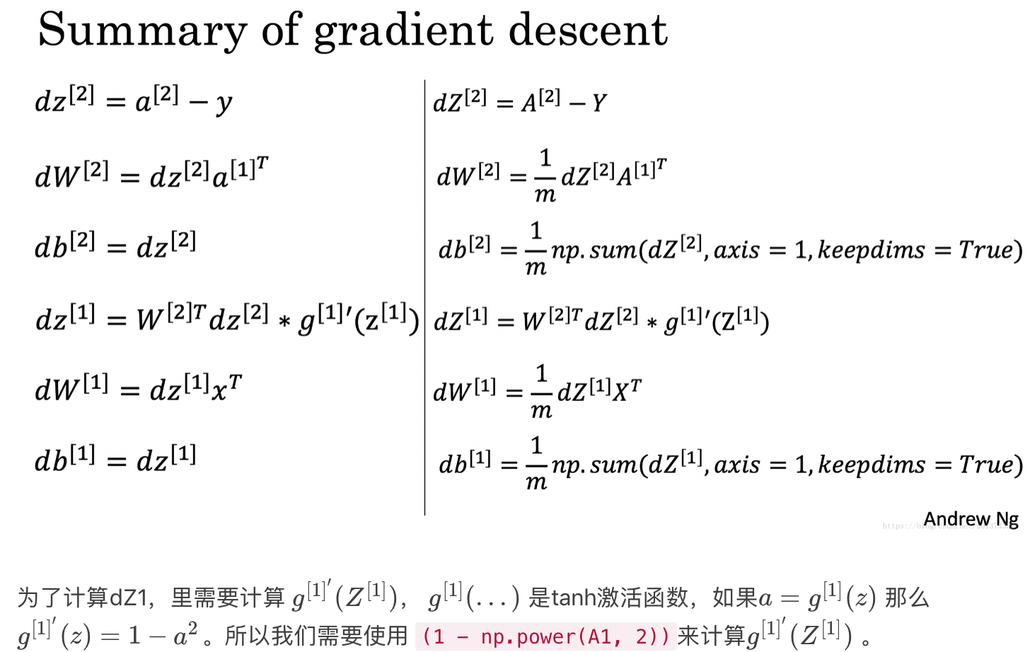
代码:
def backward_propagation(parameters,cache,X,Y):
    """
    使用上述说明搭建反向传播函数。

    参数:
     parameters - 包含我们的参数的一个字典类型的变量。
     cache - 包含“Z1”,“A1”,“Z2”和“A2”的字典类型的变量。
     X - 输入数据,维度为(2,数量)
     Y - “True”标签,维度为(1,数量)

    返回:
     grads - 包含W和b的导数一个字典类型的变量。
    """
    m = X.shape[1]

    W1 = parameters["W1"]
    W2 = parameters["W2"]

    A1 = cache["A1"]
    A2 = cache["A2"]

    dZ2= A2 - Y
    dW2 = (1 / m) * np.dot(dZ2, A1.T)
    db2 = (1 / m) * np.sum(dZ2, axis=1, keepdims=True)
    dZ1 = np.multiply(np.dot(W2.T, dZ2), 1 - np.power(A1, 2))
    dW1 = (1 / m) * np.dot(dZ1, X.T)
    db1 = (1 / m) * np.sum(dZ1, axis=1, keepdims=True)
    grads = {"dW1": dW1,
             "db1": db1,
             "dW2": dW2,
             "db2": db2 }

    return grads

#测试backward_propagation
print("=========================测试backward_propagation=========================")

def backward_propagation_test_case():
    np.random.seed(1)
    X_assess = np.random.randn(2, 3) #随机生成与上面相同的输入X
    Y_assess = np.random.randn(1, 3) #随机生成与上面相同的输出Y
    parameters = {'W1': np.array([[-0.00416758, -0.00056267], #将之前测试初始化参数时得到的值作为参数
        [-0.02136196,  0.01640271],
        [-0.01793436, -0.00841747],
        [ 0.00502881, -0.01245288]]),
     'W2': np.array([[-0.01057952, -0.00909008,  0.00551454,  0.02292208]]),
     'b1': np.array([[ 0.],
        [ 0.],
        [ 0.],
        [ 0.]]),
     'b2': np.array([[ 0.]])}

    cache = {'A1': np.array([[-0.00616578,  0.0020626 ,  0.00349619], #之前前向传播时存储在cache中的值
         [-0.05225116,  0.02725659, -0.02646251],
         [-0.02009721,  0.0036869 ,  0.02883756],
         [ 0.02152675, -0.01385234,  0.02599885]]),
  'A2': np.array([[ 0.5002307 ,  0.49985831,  0.50023963]]),
  'Z1': np.array([[-0.00616586,  0.0020626 ,  0.0034962 ],
         [-0.05229879,  0.02726335, -0.02646869],
         [-0.02009991,  0.00368692,  0.02884556],
         [ 0.02153007, -0.01385322,  0.02600471]]),
  'Z2': np.array([[ 0.00092281, -0.00056678,  0.00095853]])}
    return parameters, cache, X_assess, Y_assess

parameters, cache, X_assess, Y_assess = backward_propagation_test_case()

grads = backward_propagation(parameters, cache, X_assess, Y_assess)
print ("dW1 = "+ str(grads["dW1"]))
print ("db1 = "+ str(grads["db1"]))
print ("dW2 = "+ str(grads["dW2"]))
print ("db2 = "+ str(grads["db2"]))
返回:
=========================测试backward_propagation=========================
dW1 = [[ 0.01018708 -0.00708701]
 [ 0.00873447 -0.0060768 ]
 [-0.00530847  0.00369379]
 [-0.02206365  0.01535126]]
db1 = [[-0.00069728]
 [-0.00060606]
 [ 0.000364  ]
 [ 0.00151207]]
dW2 = [[ 0.00363613  0.03153604  0.01162914 -0.01318316]]
db2 = [[0.06589489]]
反向传播完成了,我们开始对参数进行更新
8.更新参数w,b
我们需要使用(dW1, db1, dW2, db2)来更新(W1, b1, W2, b2)
更新算法如下:
θ=θ−α(∂J/∂θ)
- α:学习速率
- θ :参数
def update_parameters(parameters,grads,learning_rate=1.2):
    """
    使用上面给出的梯度下降更新规则更新参数

    参数:
     parameters - 包含参数的字典类型的变量。
     grads - 包含导数值的字典类型的变量。
     learning_rate - 学习速率

    返回:
     parameters - 包含更新参数的字典类型的变量。
    """
    W1,W2 = parameters["W1"],parameters["W2"]
    b1,b2 = parameters["b1"],parameters["b2"]

    dW1,dW2 = grads["dW1"],grads["dW2"]
    db1,db2 = grads["db1"],grads["db2"]

    W1 = W1 - learning_rate * dW1
    b1 = b1 - learning_rate * db1
    W2 = W2 - learning_rate * dW2
    b2 = b2 - learning_rate * db2

    parameters = {"W1": W1,
                  "b1": b1,
                  "W2": W2,
                  "b2": b2}

    return parameters

#测试update_parameters
print("=========================测试update_parameters=========================")

def update_parameters_test_case():
    parameters = {'W1': np.array([[-0.00615039,  0.0169021 ], #将之前测试初始化参数时得到的值作为参数
        [-0.02311792,  0.03137121],
        [-0.0169217 , -0.01752545],
        [ 0.00935436, -0.05018221]]),
 'W2': np.array([[-0.0104319 , -0.04019007,  0.01607211,  0.04440255]]),
 'b1': np.array([[ -8.97523455e-07],
        [  8.15562092e-06],
        [  6.04810633e-07],
        [ -2.54560700e-06]]),
 'b2': np.array([[  9.14954378e-05]])}

    grads = {'dW1': np.array([[ 0.00023322, -0.00205423],
        [ 0.00082222, -0.00700776],
        [-0.00031831,  0.0028636 ],
        [-0.00092857,  0.00809933]]),
 'dW2': np.array([[ -1.75740039e-05,   3.70231337e-03,  -1.25683095e-03,
          -2.55715317e-03]]),
 'db1': np.array([[  1.05570087e-07],
        [ -3.81814487e-06],
        [ -1.90155145e-07],
        [  5.46467802e-07]]),
 'db2': np.array([[ -1.08923140e-05]])}
    return parameters, grads


parameters, grads = update_parameters_test_case()
parameters = update_parameters(parameters, grads)

print("W1 = " + str(parameters["W1"]))
print("b1 = " + str(parameters["b1"]))
print("W2 = " + str(parameters["W2"]))
print("b2 = " + str(parameters["b2"]))
9.整合上面的所有函数
使神经网络模型以正确的顺序使用先前的函数功能,整合在nn_model()函数中
def nn_model(X,Y,n_h,num_iterations,print_cost=False):
    """
    参数:
        X - 数据集,维度为(2,示例数)
        Y - 标签,维度为(1,示例数)
        n_h - 隐藏层的数量
        num_iterations - 梯度下降循环中的迭代次数
        print_cost - 如果为True,则每1000次迭代打印一次成本数值

    返回:
        parameters - 模型学习的参数,它们可以用来进行预测。
     """

    np.random.seed(3) #指定随机种子
    n_x = layer_sizes(X, Y)[0]
    n_y = layer_sizes(X, Y)[2]

    parameters = initialize_parameters(n_x,n_h,n_y)
    W1 = parameters["W1"]
    b1 = parameters["b1"]
    W2 = parameters["W2"]
    b2 = parameters["b2"]

    for i in range(num_iterations): #多次迭代,更新w,b,求出相应的成本函数
        A2 , cache = forward_propagation(X,parameters) #先前向传播,得到结果A2以及将相应的数据存储到cache中
        cost = compute_cost(A2,Y,parameters) #根据得到的结果A2和真正的结果Y去计算成本
        grads = backward_propagation(parameters,cache,X,Y) #然后计算相应参数的梯度
        parameters = update_parameters(parameters,grads,learning_rate = 0.5) #根据梯度去更新参数

        if print_cost:
            if i%1000 == 0: #1000次迭代后输出一次成本查看成本的变化
                print("第 ",i," 次循环,成本为:"+str(cost))
    return parameters
10.预测
使用上面训练好的参数w,b对测试集进行预测
输出y大于0.5则为蓝色,小于0.5则为红色
def predict(parameters,X):
    """
    使用学习的参数,为X中的每个示例预测一个类

    参数:
        parameters - 包含参数的字典类型的变量,这是训练好的参数
        X - 输入数据(n_x,m)

    返回
        predictions - 我们模型预测的向量(红色:0 /蓝色:1)

     """
   #使用训练好的参数去前向传播获取预测值
    A2 , cache = forward_propagation(X,parameters)
    predictions = np.round(A2)

    return predictions
11.整个代码运行
如果直接将整个函数放入jupyter notebook中总会报错:
ValueError: 'c' argument has 1 elements, which is not acceptable for use with 'x' with size 400, 'y' with size 400.
即使把planar_utils.py文件中的plot_decision_boundary()函数中的语句改成:
plt.scatter(X[0, :], X[1, :], c=np.squeeze(y), cmap=plt.cm.Spectral)
也不行,后面拆开导入就成功了:
import numpy as np
import matplotlib.pyplot as plt
from testCases import *
import sklearn
import sklearn.datasets
import sklearn.linear_model
def plot_decision_boundary(model, X, y):
    #用于绘制logistic的线形分类线
    # Set min and max values and give it some padding
    x_min, x_max = X[0, :].min() - 1, X[0, :].max() + 1
    y_min, y_max = X[1, :].min() - 1, X[1, :].max() + 1
    h = 0.01
    # Generate a grid of points with distance h between them
    xx, yy = np.meshgrid(np.arange(x_min, x_max, h), np.arange(y_min, y_max, h))
    # Predict the function value for the whole grid
    Z = model(np.c_[xx.ravel(), yy.ravel()])
    Z = Z.reshape(xx.shape)
    # Plot the contour and training examples
    plt.contourf(xx, yy, Z, cmap=plt.cm.Spectral)
    plt.ylabel('x2')
    plt.xlabel('x1')
    plt.scatter(X[0, :], X[1, :], c=np.squeeze(y), cmap=plt.cm.Spectral)
from planar_utils import sigmoid, load_planar_dataset, load_extra_datasets


np.random.seed(1) #设置一个固定的随机种子,以保证接下来的步骤中我们的结果是一致的。

X, Y = load_planar_dataset()
#plt.scatter(X[0, :], X[1, :], c=Y, s=40, cmap=plt.cm.Spectral) #绘制散点图
shape_X = X.shape
shape_Y = Y.shape
m = Y.shape[1]  # 训练集里面的数量

print ("X的维度为: " + str(shape_X))
print ("Y的维度为: " + str(shape_Y))
print ("数据集里面的数据有:" + str(m) + " 个")

def layer_sizes(X , Y):
    """
    参数:
     X - 输入数据集,维度为(输入的数量,训练/测试的数量)
     Y - 标签,维度为(输出的数量,训练/测试数量)

    返回:
     n_x - 输入层的数量
     n_h - 隐藏层的数量
     n_y - 输出层的数量
    """
    n_x = X.shape[0] #输入层
    n_h = 4 #,隐藏层,硬编码为4
    n_y = Y.shape[0] #输出层

    return (n_x,n_h,n_y)

def initialize_parameters( n_x , n_h ,n_y):
    """
    参数:
        n_x - 输入节点的数量
        n_h - 隐藏层节点的数量
        n_y - 输出层节点的数量

    返回:
        parameters - 包含参数的字典:
            W1 - 权重矩阵,维度为(n_h,n_x)
            b1 - 偏向量,维度为(n_h,1)
            W2 - 权重矩阵,维度为(n_y,n_h)
            b2 - 偏向量,维度为(n_y,1)

    """
    np.random.seed(2) #指定一个随机种子,以便你的输出与我们的一样。
    W1 = np.random.randn(n_h,n_x) * 0.01
    b1 = np.zeros(shape=(n_h, 1))
    W2 = np.random.randn(n_y,n_h) * 0.01
    b2 = np.zeros(shape=(n_y, 1))

    #使用断言确保我的数据格式是正确的
    assert(W1.shape == ( n_h , n_x ))
    assert(b1.shape == ( n_h , 1 ))
    assert(W2.shape == ( n_y , n_h ))
    assert(b2.shape == ( n_y , 1 ))

    parameters = {"W1" : W1,
                  "b1" : b1,
                  "W2" : W2,
                  "b2" : b2 }

    return parameters

def forward_propagation( X , parameters ):
    """
    参数:
         X - 维度为(n_x,m)的输入数据。
         parameters - 初始化函数(initialize_parameters)的输出

    返回:
         A2 - 使用sigmoid()函数计算的第二次激活后的数值
         cache - 包含“Z1”,“A1”,“Z2”和“A2”的字典类型变量
     """
    W1 = parameters["W1"]
    b1 = parameters["b1"]
    W2 = parameters["W2"]
    b2 = parameters["b2"]
    #前向传播计算A2
    Z1 = np.dot(W1 , X) + b1
    A1 = np.tanh(Z1)
    Z2 = np.dot(W2 , A1) + b2
    A2 = sigmoid(Z2)
    #使用断言确保我的数据格式是正确的
    assert(A2.shape == (1,X.shape[1]))
    cache = {"Z1": Z1,
             "A1": A1,
             "Z2": Z2,
             "A2": A2}

    return (A2, cache)

def compute_cost(A2,Y,parameters):
    """
    计算方程(6)中给出的交叉熵成本,

    参数:
         A2 - 使用sigmoid()函数计算的第二次激活后的数值
         Y - "True"标签向量,维度为(1,数量)
         parameters - 一个包含W1,B1,W2和B2的字典类型的变量

    返回:
         成本 - 交叉熵成本给出方程(13)
    """

    m = Y.shape[1]
    W1 = parameters["W1"]
    W2 = parameters["W2"]

    #计算成本
    logprobs = logprobs = np.multiply(np.log(A2), Y) + np.multiply((1 - Y), np.log(1 - A2))
    cost = - np.sum(logprobs) / m
    cost = float(np.squeeze(cost))

    assert(isinstance(cost,float))

    return cost

def backward_propagation(parameters,cache,X,Y):
    """
    使用上述说明搭建反向传播函数。

    参数:
     parameters - 包含我们的参数的一个字典类型的变量。
     cache - 包含“Z1”,“A1”,“Z2”和“A2”的字典类型的变量。
     X - 输入数据,维度为(2,数量)
     Y - “True”标签,维度为(1,数量)

    返回:
     grads - 包含W和b的导数一个字典类型的变量。
    """
    m = X.shape[1]

    W1 = parameters["W1"]
    W2 = parameters["W2"]

    A1 = cache["A1"]
    A2 = cache["A2"]

    dZ2= A2 - Y
    dW2 = (1 / m) * np.dot(dZ2, A1.T)
    db2 = (1 / m) * np.sum(dZ2, axis=1, keepdims=True)
    dZ1 = np.multiply(np.dot(W2.T, dZ2), 1 - np.power(A1, 2))
    dW1 = (1 / m) * np.dot(dZ1, X.T)
    db1 = (1 / m) * np.sum(dZ1, axis=1, keepdims=True)
    grads = {"dW1": dW1,
             "db1": db1,
             "dW2": dW2,
             "db2": db2 }

    return grads

def update_parameters(parameters,grads,learning_rate=1.2):
    """
    使用上面给出的梯度下降更新规则更新参数

    参数:
     parameters - 包含参数的字典类型的变量。
     grads - 包含导数值的字典类型的变量。
     learning_rate - 学习速率

    返回:
     parameters - 包含更新参数的字典类型的变量。
    """
    W1,W2 = parameters["W1"],parameters["W2"]
    b1,b2 = parameters["b1"],parameters["b2"]

    dW1,dW2 = grads["dW1"],grads["dW2"]
    db1,db2 = grads["db1"],grads["db2"]

    W1 = W1 - learning_rate * dW1
    b1 = b1 - learning_rate * db1
    W2 = W2 - learning_rate * dW2
    b2 = b2 - learning_rate * db2

    parameters = {"W1": W1,
                  "b1": b1,
                  "W2": W2,
                  "b2": b2}

    return parameters

def nn_model(X,Y,n_h,num_iterations,print_cost=False):
    """
    参数:
        X - 数据集,维度为(2,示例数)
        Y - 标签,维度为(1,示例数)
        n_h - 隐藏层的数量
        num_iterations - 梯度下降循环中的迭代次数
        print_cost - 如果为True,则每1000次迭代打印一次成本数值

    返回:
        parameters - 模型学习的参数,它们可以用来进行预测。
     """

    np.random.seed(3) #指定随机种子
    n_x = layer_sizes(X, Y)[0]
    n_y = layer_sizes(X, Y)[2]

    parameters = initialize_parameters(n_x,n_h,n_y)
    W1 = parameters["W1"]
    b1 = parameters["b1"]
    W2 = parameters["W2"]
    b2 = parameters["b2"]

    for i in range(num_iterations): #多次迭代,更新w,b,求出相应的成本函数
        A2 , cache = forward_propagation(X,parameters) #先前向传播,得到结果A2以及将相应的数据存储到cache中
        cost = compute_cost(A2,Y,parameters) #根据得到的结果A2和真正的结果Y去计算成本
        grads = backward_propagation(parameters,cache,X,Y) #然后计算相应参数的梯度
        parameters = update_parameters(parameters,grads,learning_rate = 0.5) #根据梯度去更新参数

        if print_cost:
            if i%1000 == 0: #1000次迭代后输出一次成本查看成本的变化
                print("第 ",i," 次循环,成本为:"+str(cost))
    return parameters

def predict(parameters,X):
    """
    使用学习的参数w,b,为X中的每个示例预测一个类

    参数:
        parameters - 包含参数的字典类型的变量。
        X - 输入数据(n_x,m)

    返回
        predictions - 我们模型预测的向量(红色:0 /蓝色:1)

     """
    A2 , cache = forward_propagation(X,parameters)
    predictions = np.round(A2)

    return predictions
返回:
X的维度为: (2, 400)
Y的维度为: (1, 400)
数据集里面的数据有:400 个
然后运行:
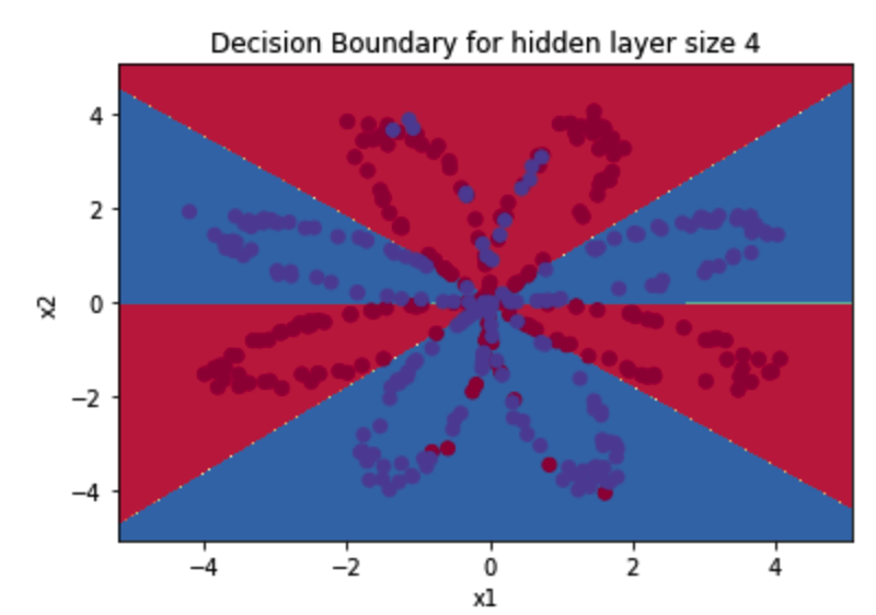
parameters = nn_model(X, Y, n_h = 4, num_iterations=10000, print_cost=True)

#绘制边界
plot_decision_boundary(lambda x: predict(parameters, x.T), X, Y)
plt.title("Decision Boundary for hidden layer size " + str(4))

predictions = predict(parameters, X)
print ('准确率: %d' % float((np.dot(Y, predictions.T) + np.dot(1 - Y, 1 - predictions.T)) / float(Y.size) * 100) + '%')
返回:
第  0  次循环,成本为:0.6930480201239823
第  1000  次循环,成本为:0.3098018601352803
第  2000  次循环,成本为:0.2924326333792646
第  3000  次循环,成本为:0.2833492852647412
第  4000  次循环,成本为:0.27678077562979253
第  5000  次循环,成本为:0.26347155088593194
第  6000  次循环,成本为:0.2420441312994077
第  7000  次循环,成本为:0.23552486626608765
第  8000  次循环,成本为:0.23140964509854278
第  9000  次循环,成本为:0.22846408048352365
准确率: 90%
图示为:
12.优化
1)更改隐藏层神经元数量
plt.figure(figsize=(16, 32))
hidden_layer_sizes = [1, 2, 3, 4, 5, 20, 50] #更改隐藏层数量
for i, n_h in enumerate(hidden_layer_sizes):
    plt.subplot(5, 2, i + 1)
    plt.title('Hidden Layer of size %d' % n_h)
    parameters = nn_model(X, Y, n_h, num_iterations=5000)
    plot_decision_boundary(lambda x: predict(parameters, x.T), X, Y)
    predictions = predict(parameters, X)
    accuracy = float((np.dot(Y, predictions.T) + np.dot(1 - Y, 1 - predictions.T)) / float(Y.size) * 100)
    print ("隐藏层的节点数量: {}  ,准确率: {} %".format(n_h, accuracy))
返回:
隐藏层的节点数量: 1  ,准确率: 67.25 %
隐藏层的节点数量: 2  ,准确率: 66.5 %
隐藏层的节点数量: 3  ,准确率: 89.25 %
隐藏层的节点数量: 4  ,准确率: 90.0 %
隐藏层的节点数量: 5  ,准确率: 89.75 %
隐藏层的节点数量: 20  ,准确率: 90.0 %
隐藏层的节点数量: 50  ,准确率: 89.75 %
图示:
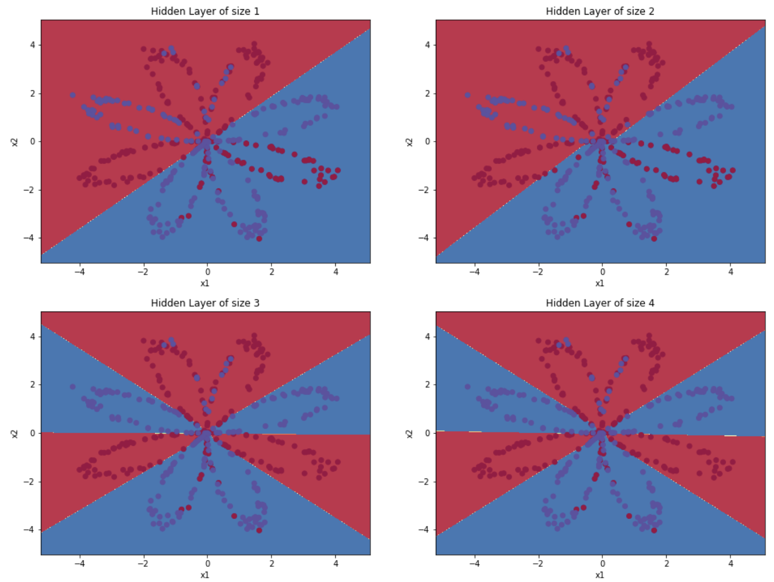
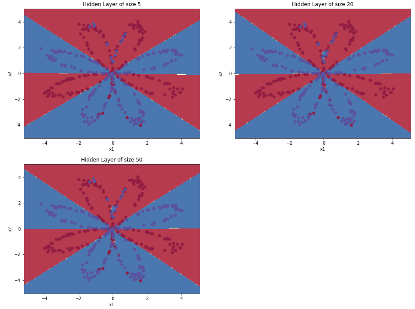
较大的模型(具有更多隐藏单元)能够更好地适应训练集,直到最终的最大模型过度拟合数据。
最好的隐藏层大小似乎在n_h = 4附近。实际上,这里的值似乎很适合数据,而且不会引起过度拟合。
我们还将在后面学习有关正则化的知识,它允许我们使用非常大的模型(如n_h = 50),而不会出现太多过度拟合。
2)如果更改的是学习率:
将函数更改为:
def nn_model(X,Y,n_h,num_iterations,lr,print_cost=False): #添加学习率lr
    """
    参数:
        X - 数据集,维度为(2,示例数)
        Y - 标签,维度为(1,示例数)
        n_h - 隐藏层的数量
        num_iterations - 梯度下降循环中的迭代次数
        print_cost - 如果为True,则每1000次迭代打印一次成本数值

    返回:
        parameters - 模型学习的参数,它们可以用来进行预测。
     """

    np.random.seed(3) #指定随机种子
    n_x = layer_sizes(X, Y)[0]
    n_y = layer_sizes(X, Y)[2]

    parameters = initialize_parameters(n_x,n_h,n_y)
    W1 = parameters["W1"]
    b1 = parameters["b1"]
    W2 = parameters["W2"]
    b2 = parameters["b2"]

    for i in range(num_iterations):
        A2 , cache = forward_propagation(X,parameters)
        cost = compute_cost(A2,Y,parameters)
        grads = backward_propagation(parameters,cache,X,Y)
        parameters = update_parameters(parameters,grads,learning_rate = lr) #学习率根据输入进行变化

        if print_cost:
            if i%1000 == 0:
                print("第 ",i," 次循环,成本为:"+str(cost))
    return parameters
测试:
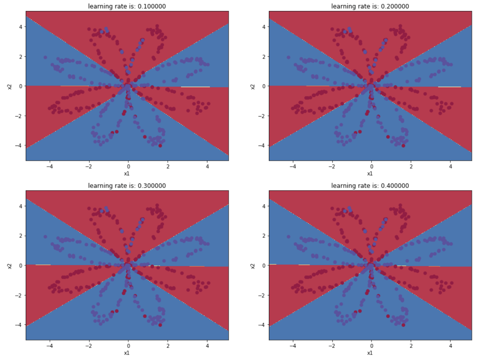
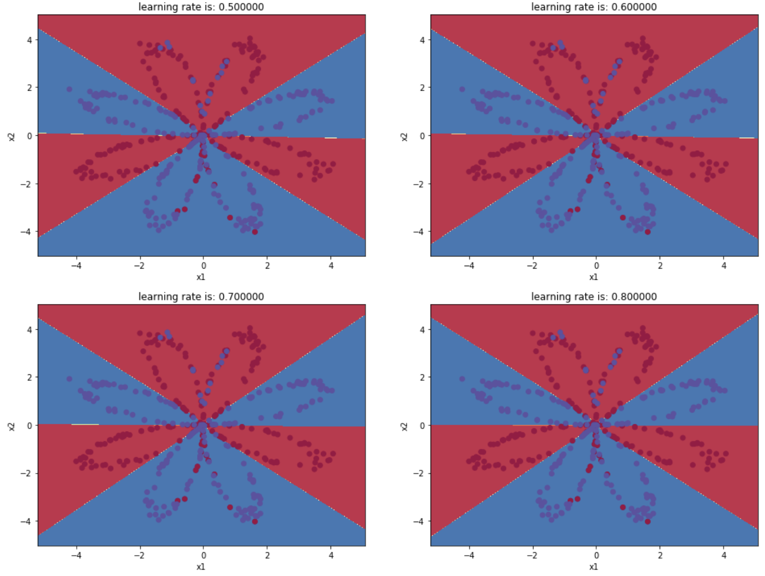
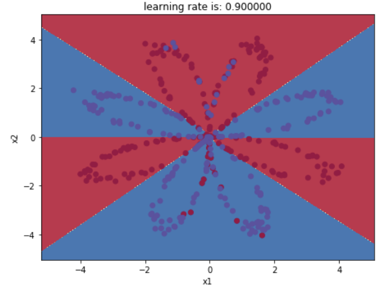
plt.figure(figsize=(16, 32))
lrs = [0.1,0.2,0.3,0.4,0.5,0.6,0.7,0.8,0.9] #更改隐藏层数量
for i, lr in enumerate(lrs):
    plt.subplot(5, 2, i + 1)
    plt.title('learning rate is: %f' % lr)
    parameters = nn_model(X, Y, n_h = 4,num_iterations=5000,lr = lr)
    plot_decision_boundary(lambda x: predict(parameters, x.T), X, Y)
    predictions = predict(parameters, X)
    accuracy = float((np.dot(Y, predictions.T) + np.dot(1 - Y, 1 - predictions.T)) / float(Y.size) * 100)
    print ("学习率为: {}  ,准确率: {} %".format(lr, accuracy))
返回:
学习率为: 0.1  ,准确率: 88.0 %
学习率为: 0.2  ,准确率: 89.25 %
学习率为: 0.3  ,准确率: 89.5 %
学习率为: 0.4  ,准确率: 89.5 %
学习率为: 0.5  ,准确率: 90.0 %
学习率为: 0.6  ,准确率: 90.25 %
学习率为: 0.7  ,准确率: 90.5 %
学习率为: 0.8  ,准确率: 90.5 %
学习率为: 0.9  ,准确率: 90.5 %
图示为: